Microbiome Analysis

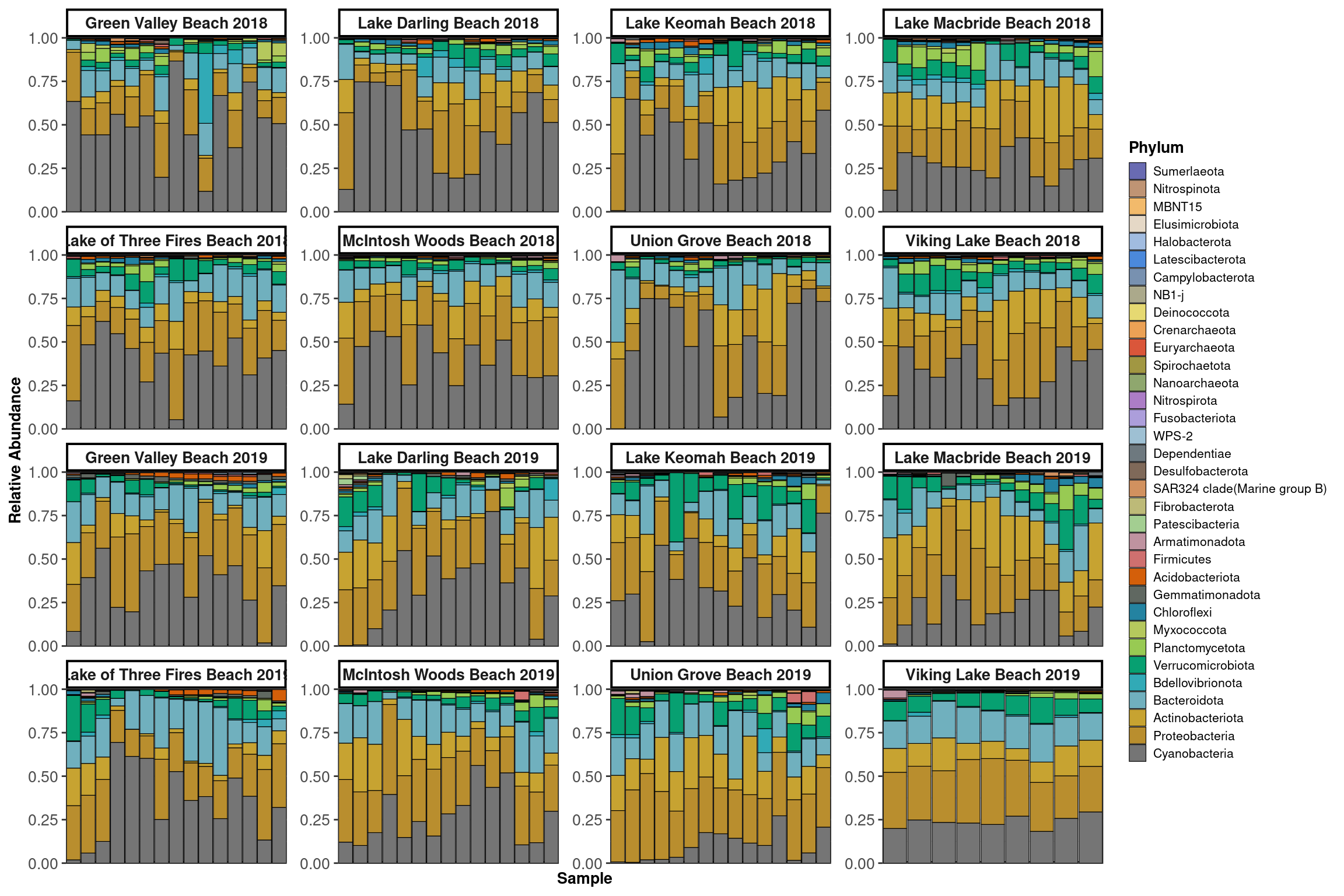
Communities

Profiles

for (risk in c('Low', 'High')){
    cat('###', risk, '<br>', '\n\n')
    profile <- phylosmith::phylogeny_profile(taxa_filter(lake_hl, "Lake_Risk", 
      risk), classification = 'Phylum', treatment = c('Location', 'Year'), 
      grid = TRUE, relative_abundance = TRUE)
    print(profile)
    cat('\n', '<br><br><br>', '\n\n')
  }

Low

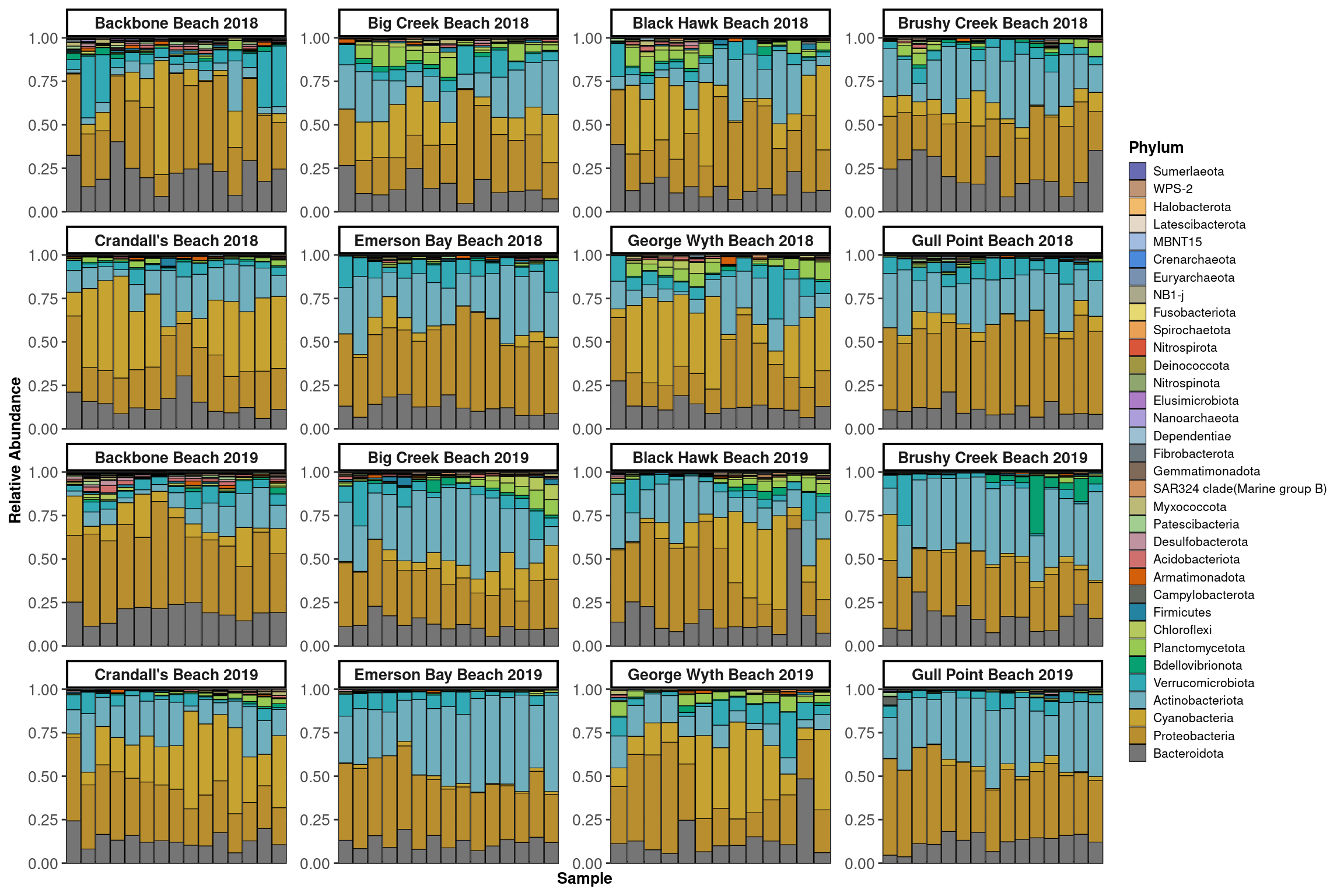
High

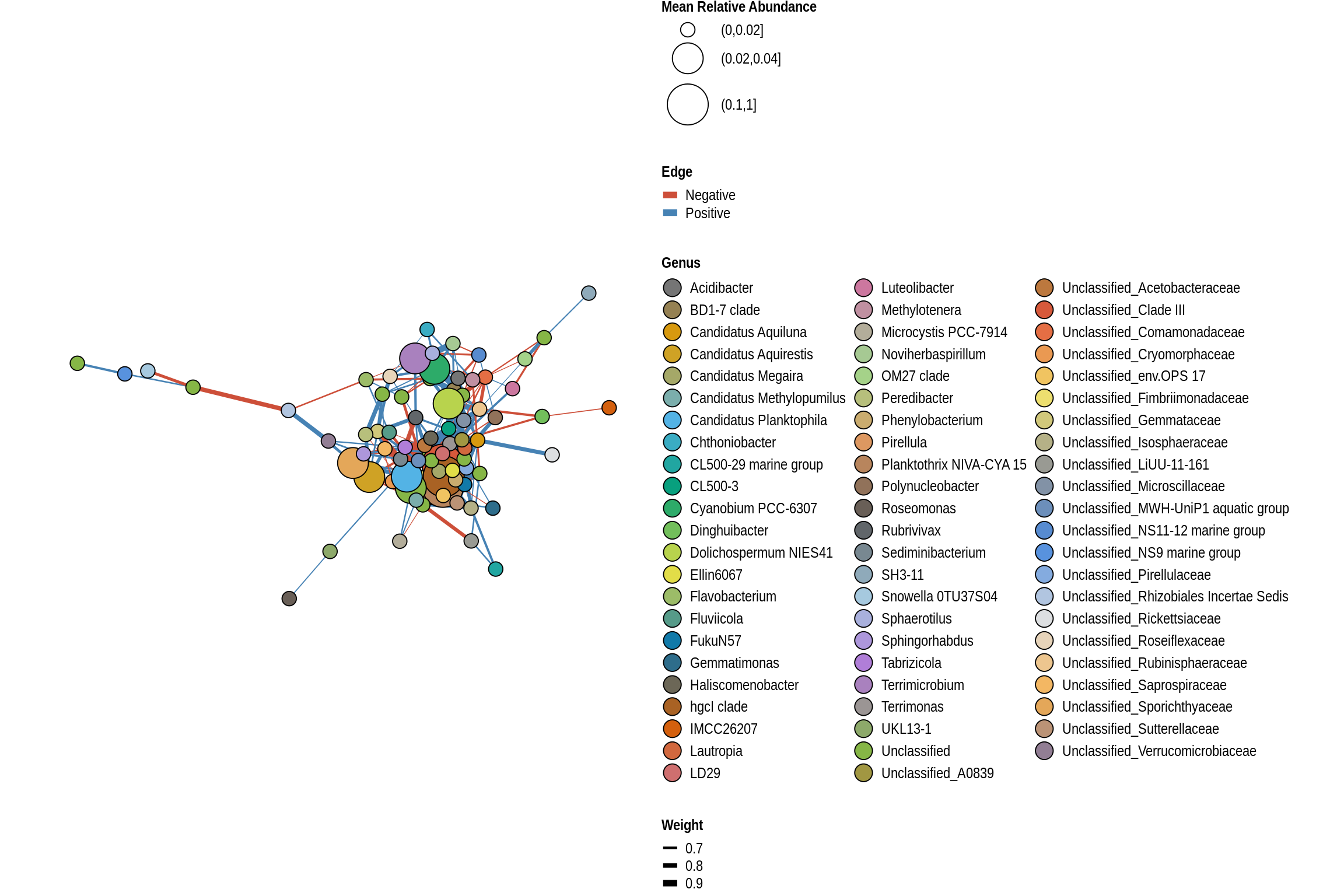
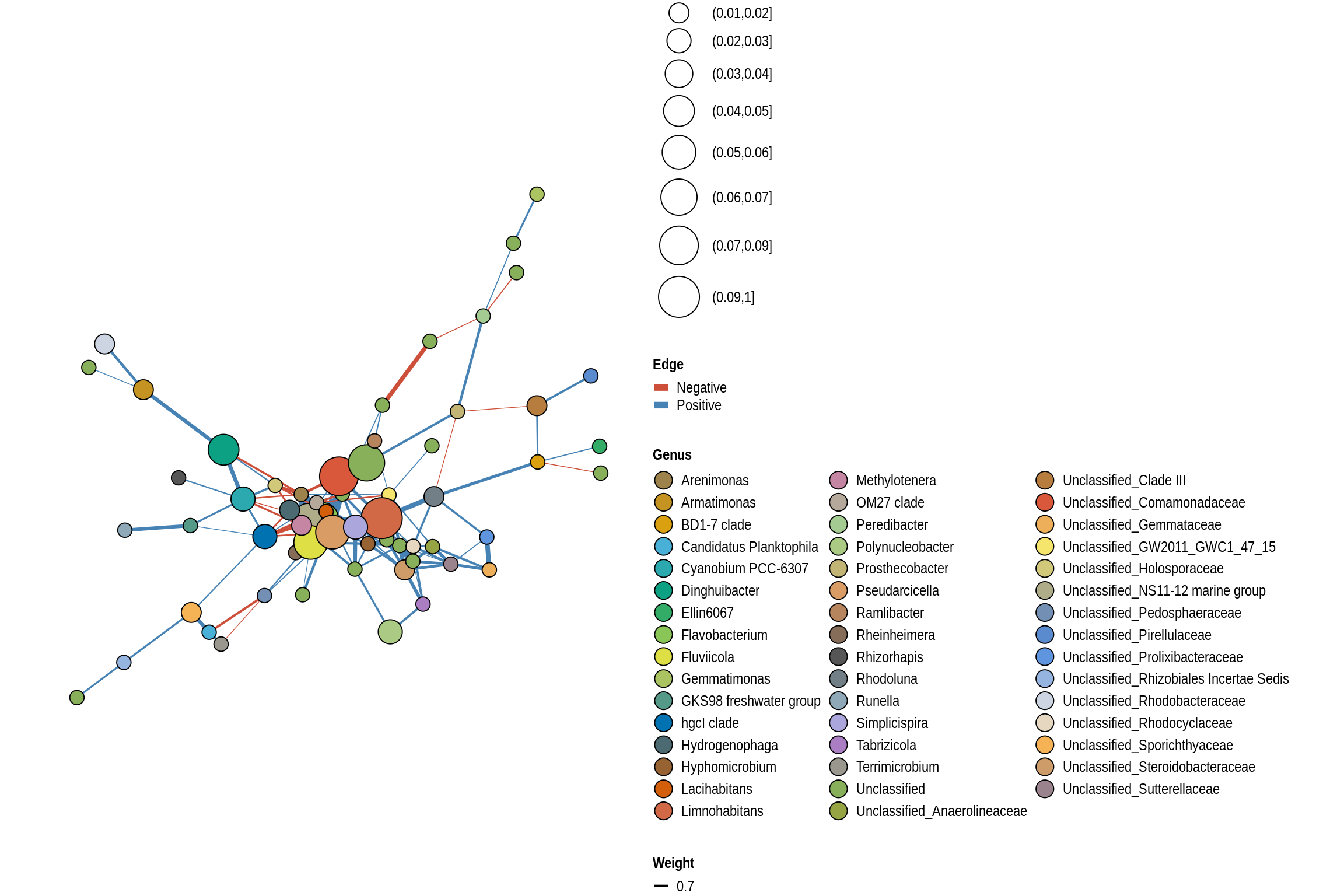
Co-Occurrences

Calculate

lake_hl_co <- taxa_filter(conglomerate_taxa(lake_hl, "Genus", TRUE, 
  use_taxonomic_names = FALSE), c("Location", "Year"), frequency = 0.25)
lake_hl_co <- co_occurrence(lake_hl_co, treatment = c("Location", "Year"))
lake_co_table <- lake_hl_co[p < 0.05]
setorder(lake_co_table, -rho)

Seperate High-Low

lake_co_table <- lake_co_table[rho < 0]
lake_co_table[,p:=NULL]
lake_co_table[, Risk := "Low"]
set(lake_co_table, unlist(sapply(high_risk_lakes, FUN=function(x)grep(x,lake_co_table$Treatment))), "Risk", "High")
lake_co_table <- lake_co_table[, c("X", "Y", "Treatment", "Risk", "rho")]
lake_co_table[,Edge := paste(X,Y,sep="-")]
high <- lake_co_table[unlist(sapply(high_risk_lakes, FUN=function(x)grep(x,lake_co_table$Treatment))),]
low <- lake_co_table[unlist(sapply(low_risk_lakes, FUN=function(x)grep(x,lake_co_table$Treatment))),]

Lake Networks

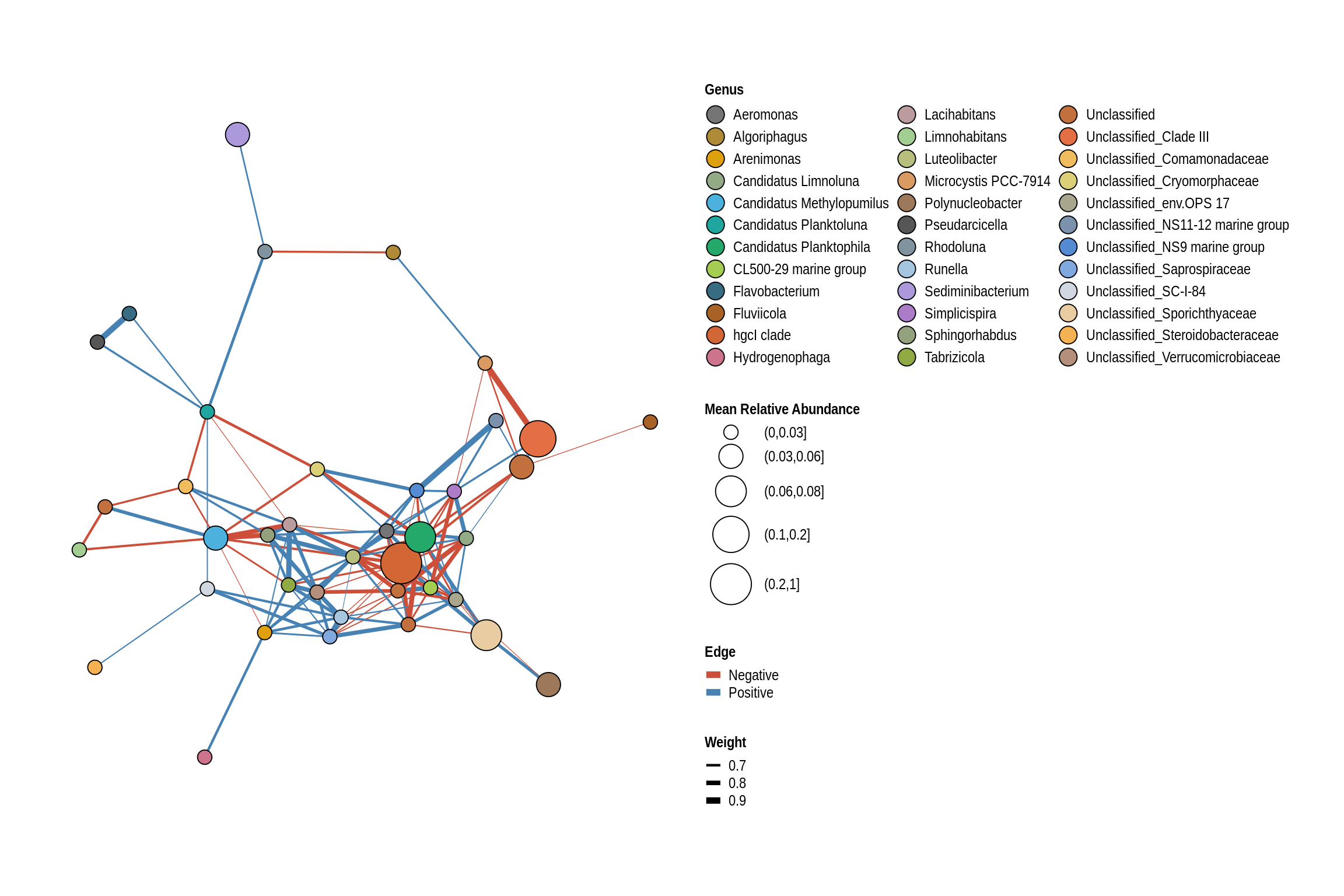
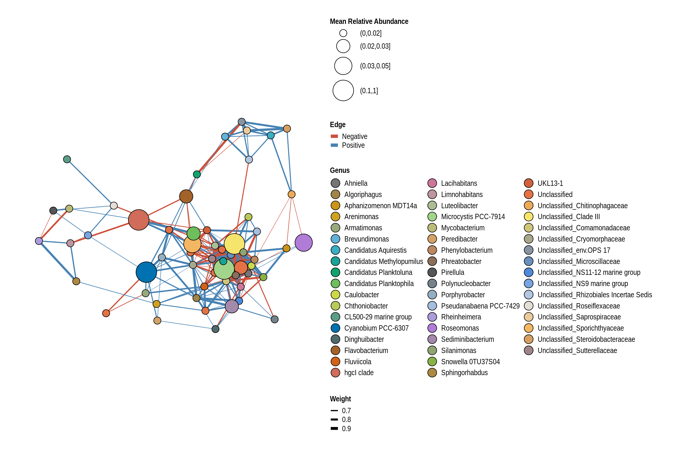
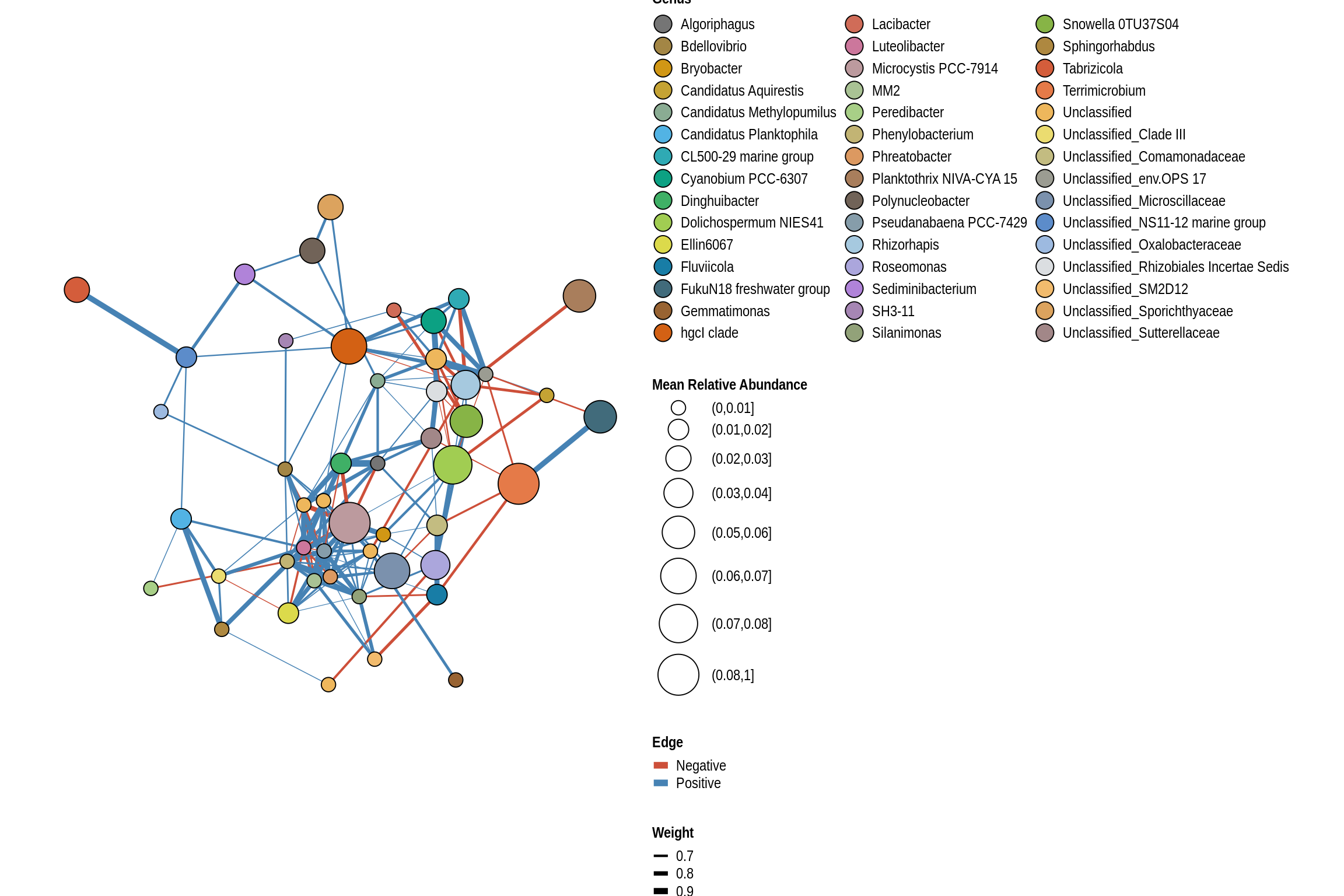
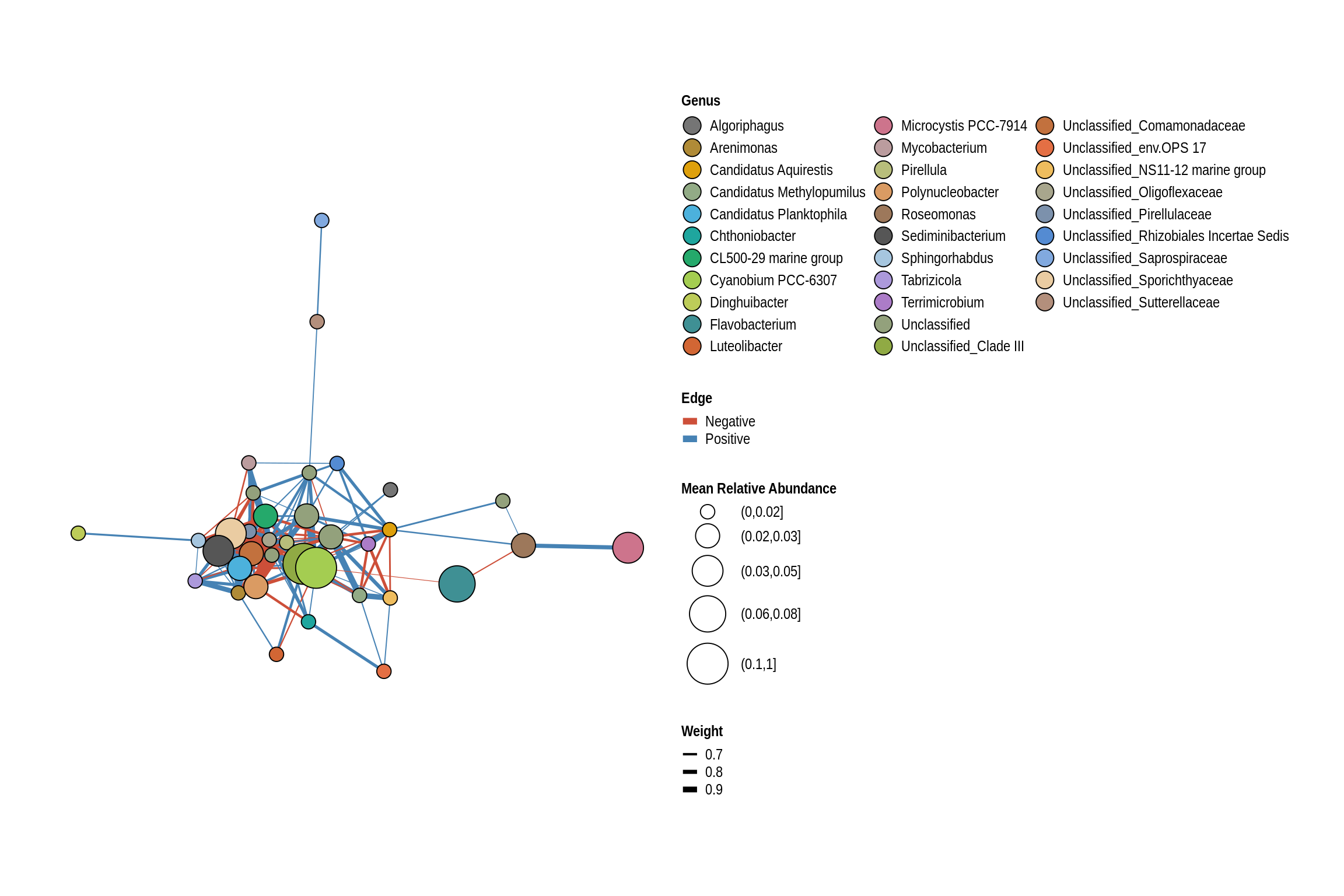
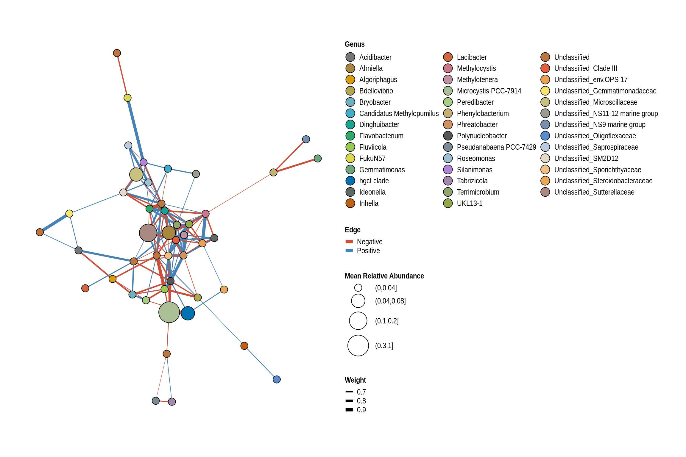
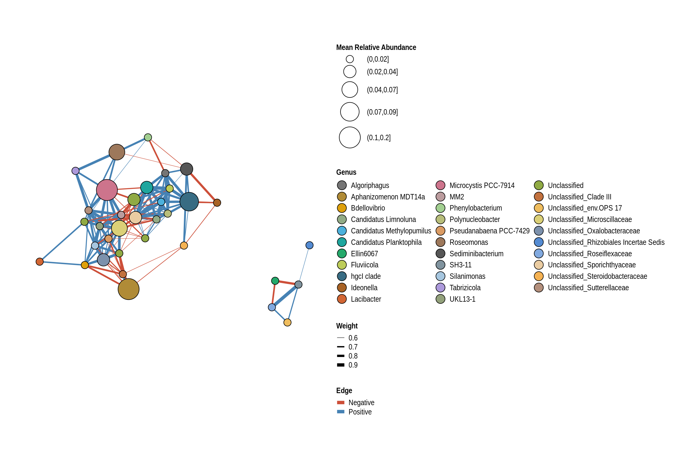
phyloseq_obj <- relative_abundance(taxa_filter(conglomerate_taxa(lake_hl, 
         "Genus", TRUE, FALSE), c("Location", "Year"), frequency = 0.25))
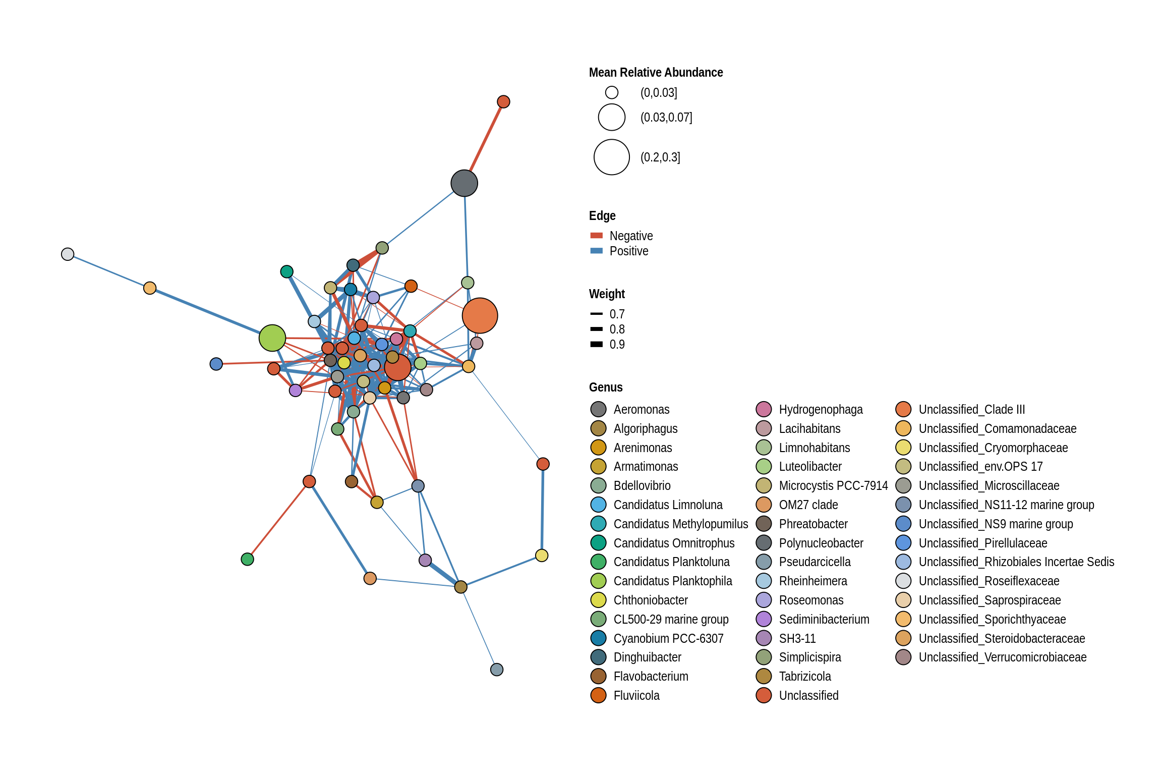
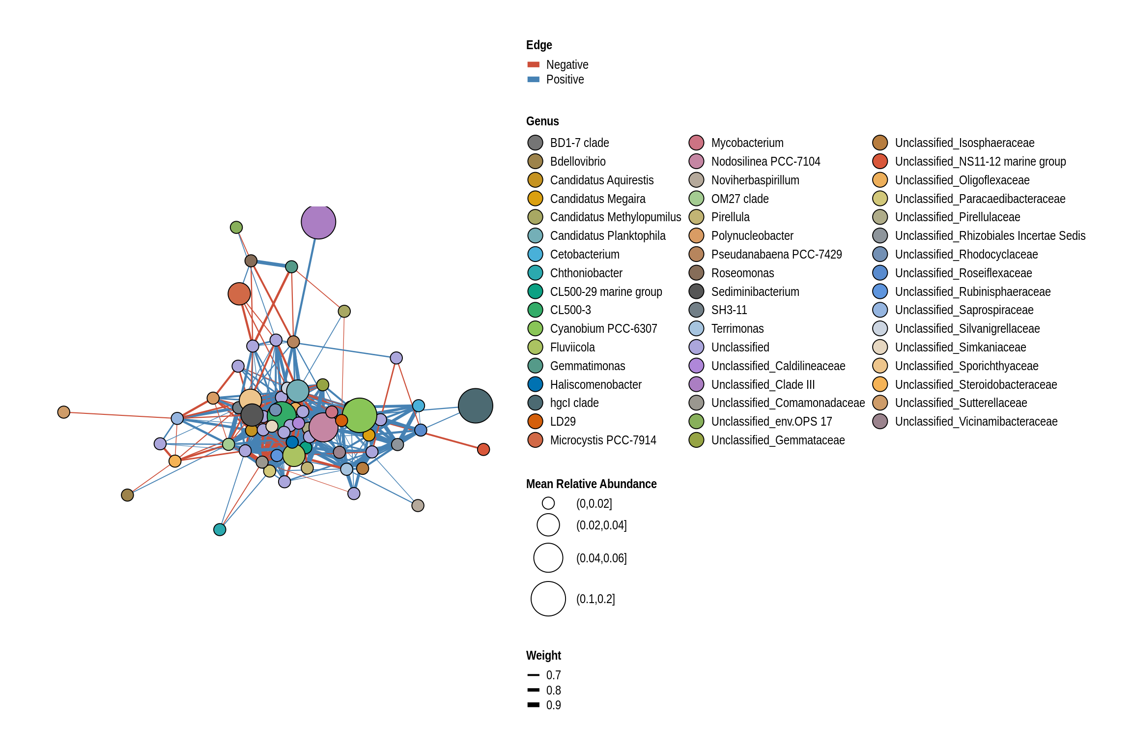
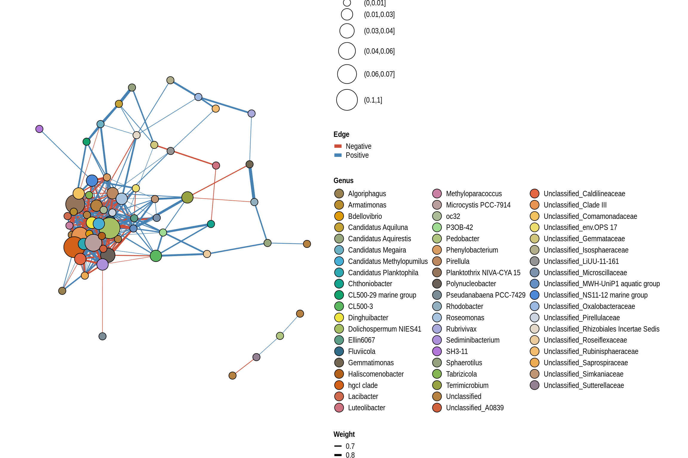
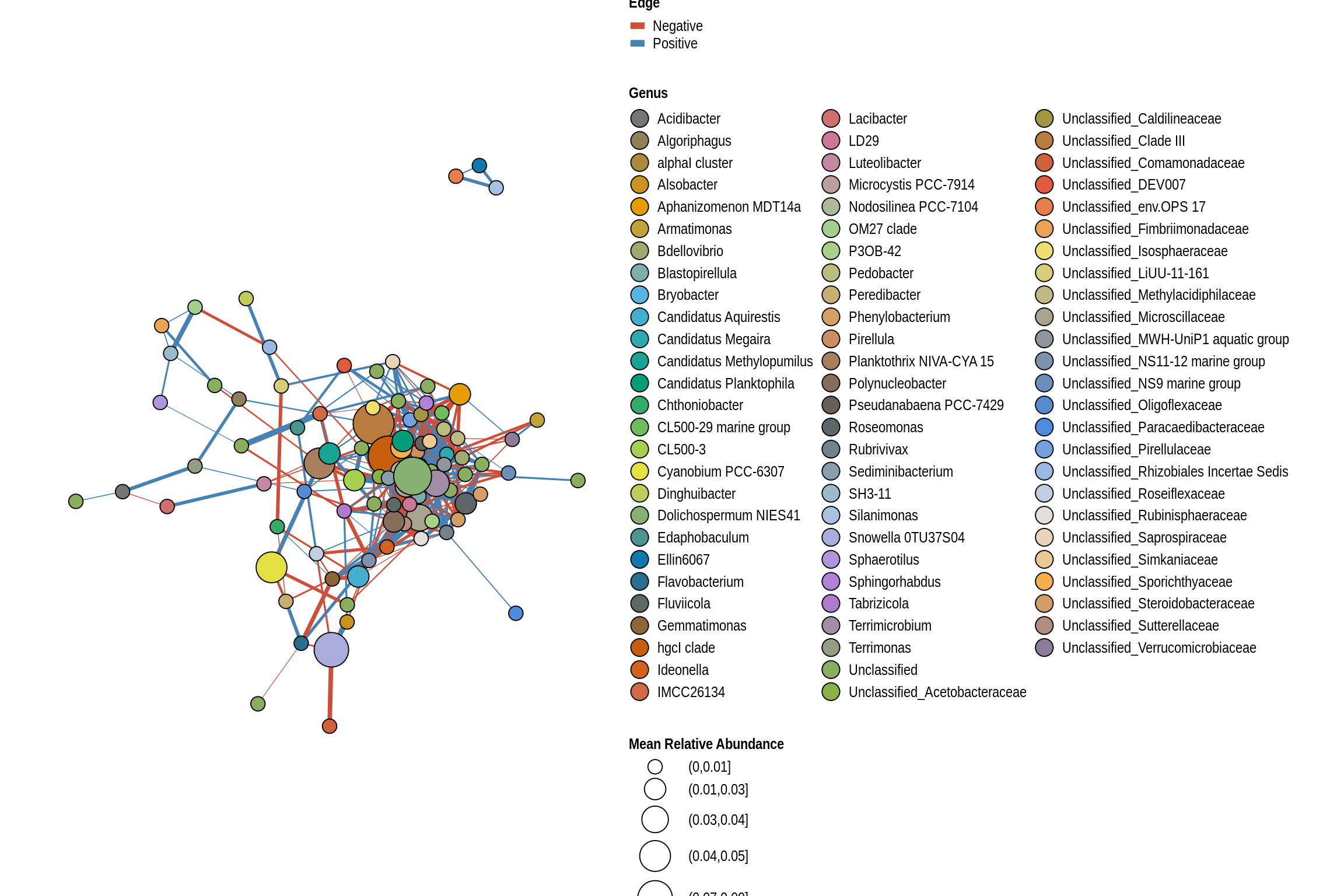
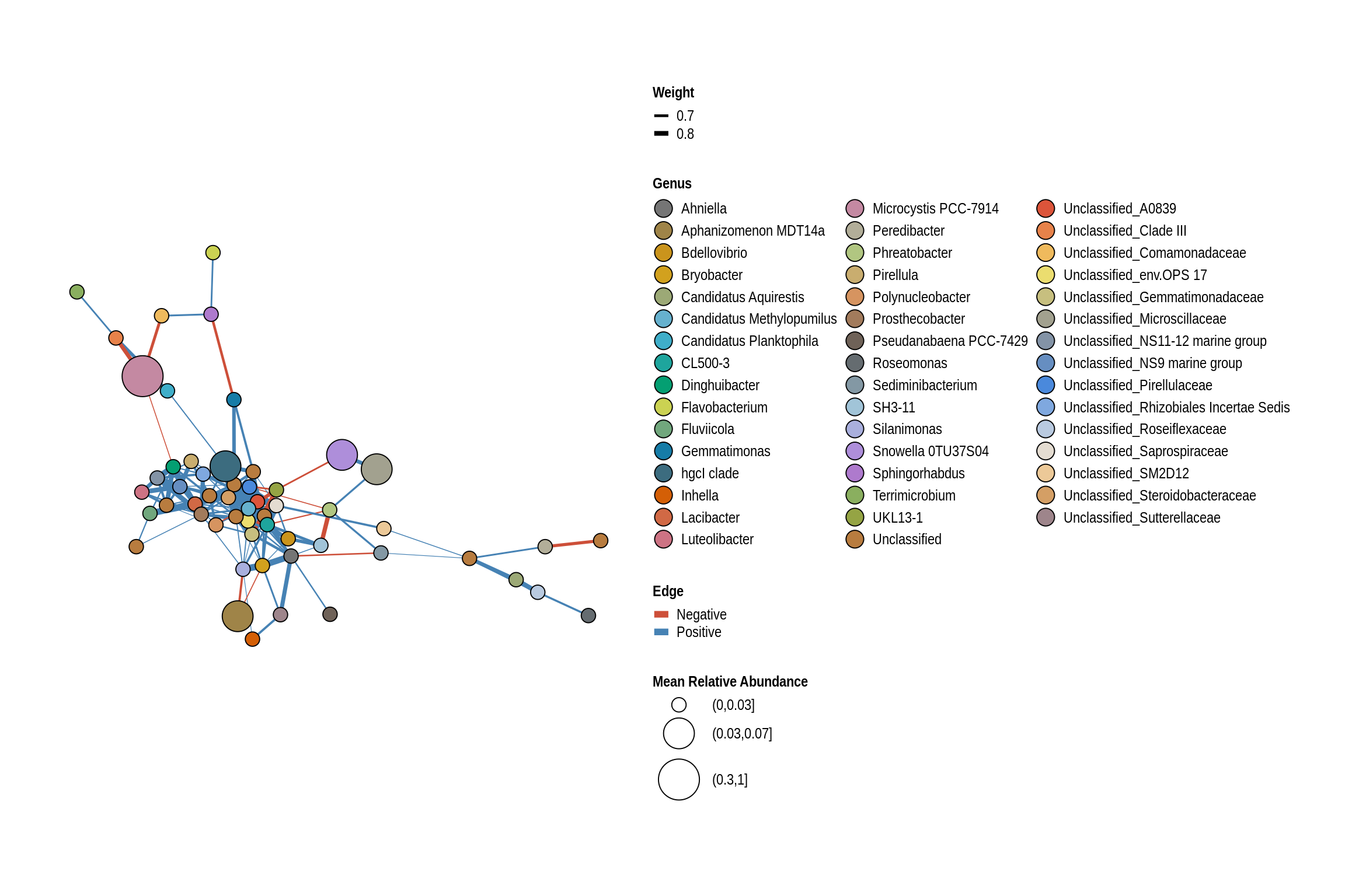
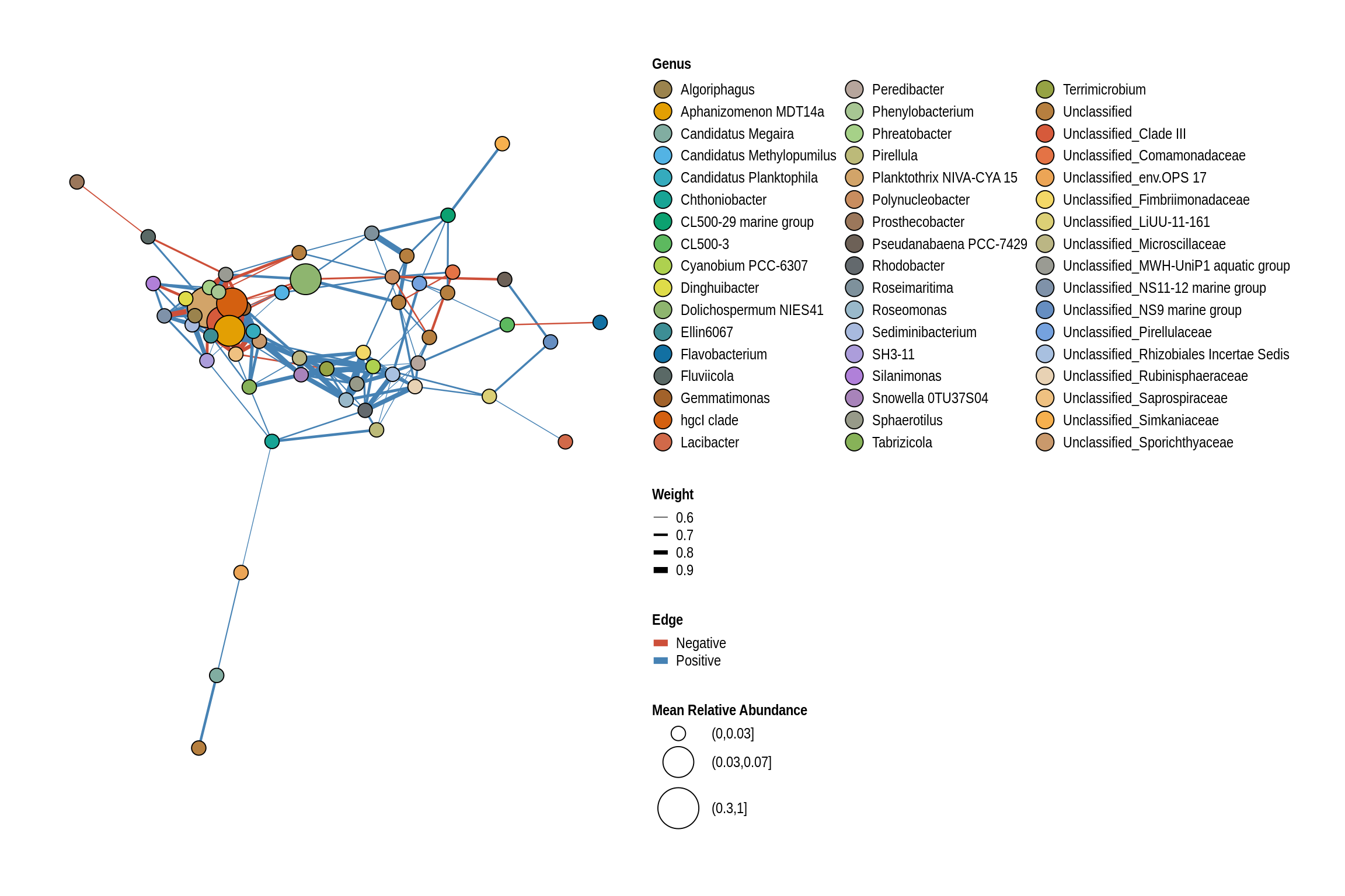
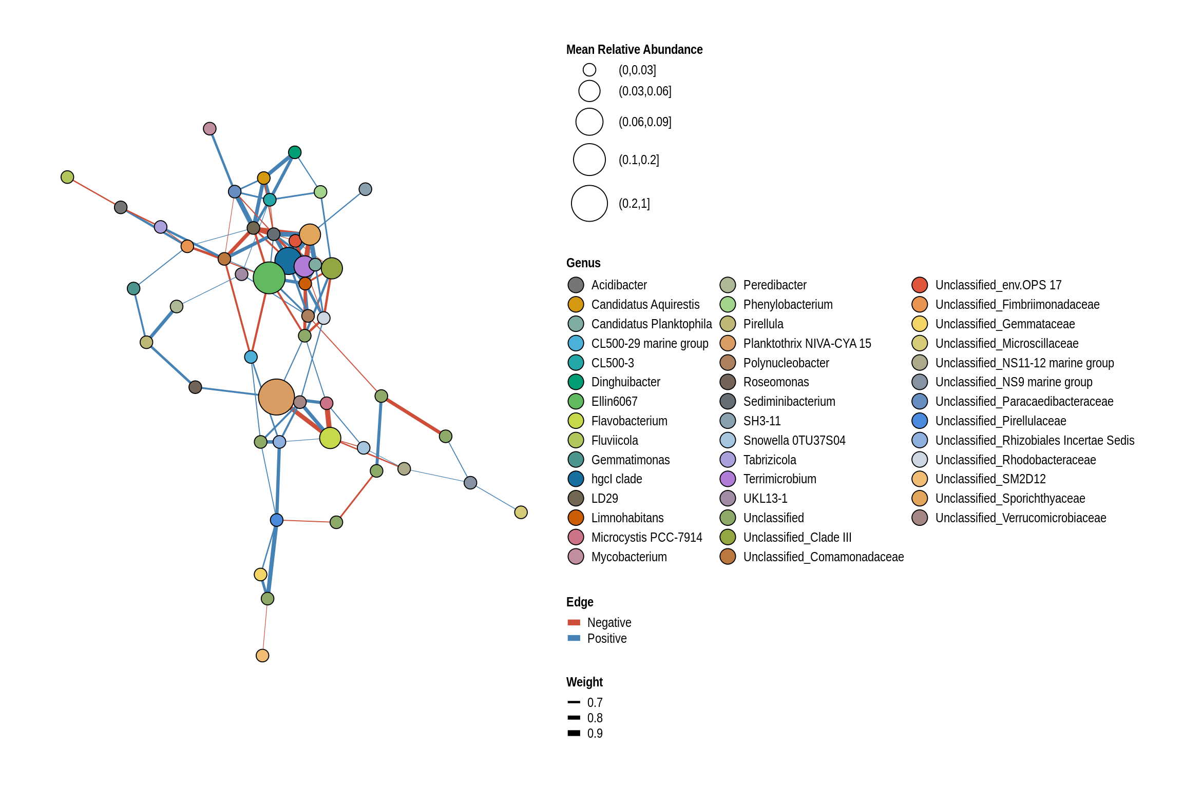
for (year in unique(metadata$Year)){
  cat('### ', year, '<br>', '\n\n')
  cat('#### Lake {.tabset}', '\n', '<br>', '\n\n')
  for (lake in unique(phyloseq_obj@sam_data$Location)){
    cat('#####', lake, '<br>', '\n\n')
    phylo_obj <- taxa_filter(phyloseq_obj, c("Location","Year"), c(lake), frequency = 0.5)
    phylo_obj <- taxa_filter(phylo_obj, c("Year"), year, frequency = 0.7)
    net <- co_occurrence_network(phylo_obj, classification = "Genus")
    print(net + guides(fill = guide_legend(ncol = 3, override.aes = list(size = 5))))
    cat('\n', '<br><br><br>', '\n\n')
  }
  cat('\n', '<br><br><br>', '\n\n')
}

2018

Lake

George Wyth Beach

McIntosh Woods Beach

Backbone Beach

Gull Point Beach

Emerson Bay Beach

Crandall’s Beach

Lake Macbride Beach

Lake Keomah Beach

Viking Lake Beach

Big Creek Beach

Black Hawk Beach

Union Grove Beach

Lake of Three Fires Beach

Green Valley Beach

Lake Darling Beach

Brushy Creek Beach

2019

Lake

George Wyth Beach

McIntosh Woods Beach

Backbone Beach

Gull Point Beach

Emerson Bay Beach

Crandall’s Beach

Lake Macbride Beach

Lake Keomah Beach

Viking Lake Beach

Big Creek Beach

Black Hawk Beach

Union Grove Beach

Lake of Three Fires Beach

Green Valley Beach

Lake Darling Beach

Brushy Creek Beach

Summary of Networks

# high_ <- high[!(Edge %in% low$Edge),]
high <- high[, .(Count = .N, rho = mean(rho)), by = c("X", "Y", "Edge")]
high <- high[Count >= 7]
setorder(high, -Count)
# low_ <- low[!(Edge %in% high$Edge),]
low <- low[, .(Count = .N, rho = mean(rho)), by = c("X", "Y", "Edge")]
low <- low[Count >= 6]
setorder(low, -Count)

Summary of Low-Risk Lakes

low

Summary of High-Risk Lakes

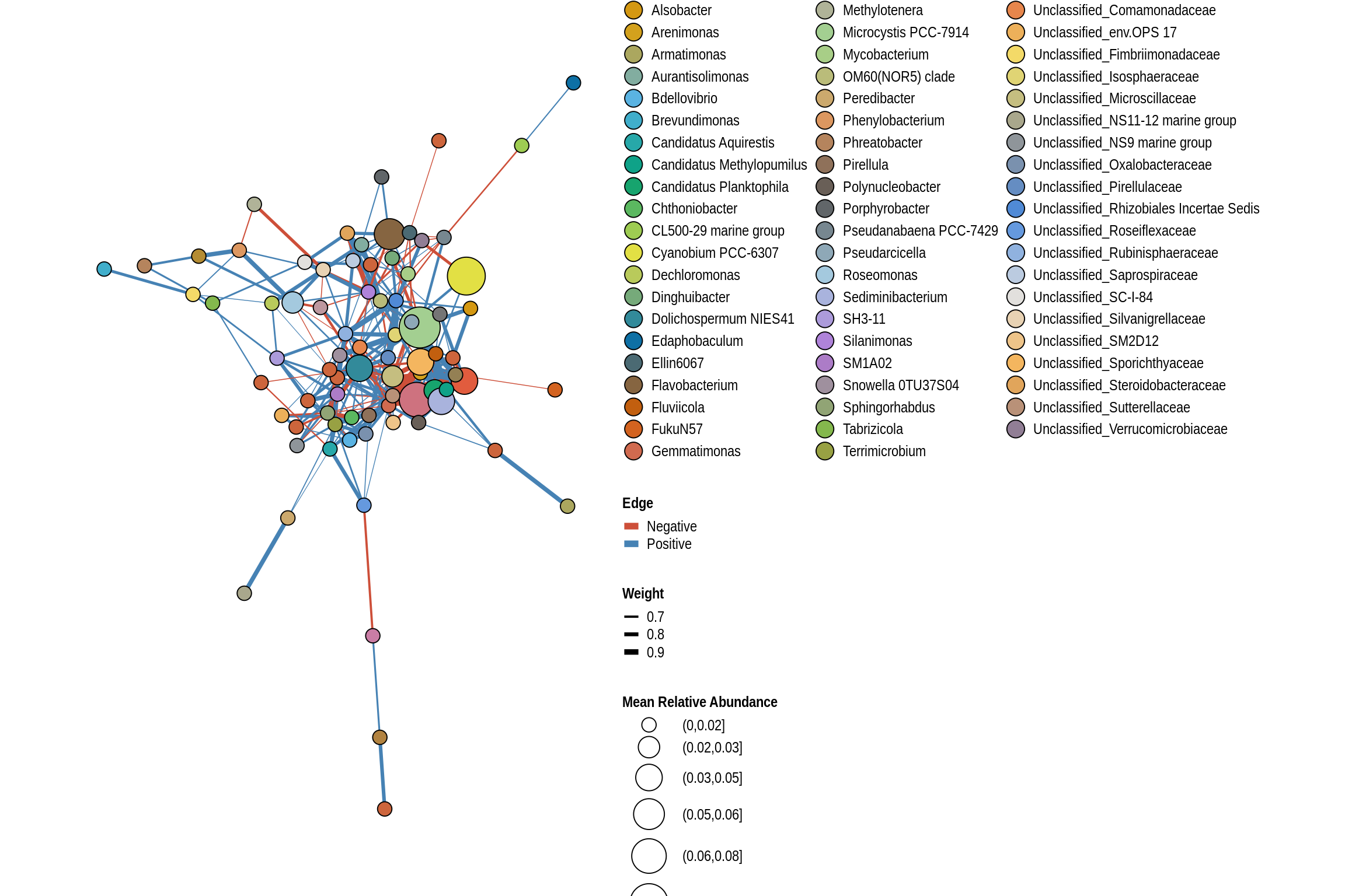
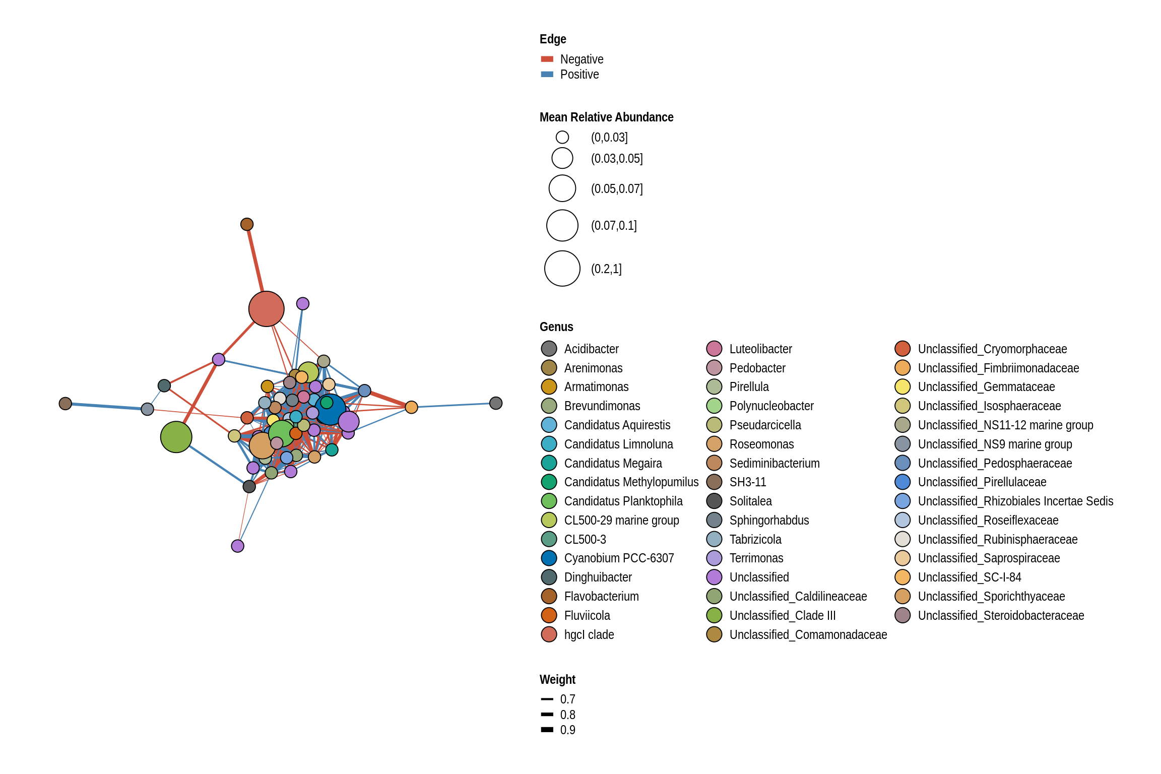
high

co_occurrence_table <- high
phyloseq_obj <- relative_abundance(conglomerate_taxa(lake_hl, "Genus", TRUE, FALSE))
nodes <- data.table(as(access(phyloseq_obj, "tax_table"), "matrix"), keep.rownames = "Node_Name")
nodes[, `Mean Relative Abundance` := phylosmith:::bin(taxa_sums(phyloseq_obj)/nsamples(phyloseq_obj), nbins = 9)]
nodes <- nodes[nodes[["Node_Name"]] %in% c(as.character(co_occurrence_table$X), 
                                           as.character(co_occurrence_table$Y)), ]
co_occurrence_table[, `:=`(Weight, abs(rho))]
node_classes <- unique(c(co_occurrence_table$X, co_occurrence_table$Y))


clusters <- cluster_fast_greedy(simplify(graph_from_data_frame(d = co_occurrence_table, vertices = nodes, directed = FALSE), remove.multiple = TRUE, remove.loops = TRUE))$membership
cluster_sizes <- table(clusters)


nodes <- nodes[clusters %in% names(cluster_sizes[cluster_sizes > 2])]
co_occurrence_table <- co_occurrence_table[X %in% nodes$Node_Name & 
                                             Y %in% nodes$Node_Name]

net <- graph_from_data_frame(d = co_occurrence_table, vertices = nodes, directed = FALSE)
layout <- ggraph::create_layout(net, layout = "igraph", algorithm = "fr")

cluster <- cluster_fast_greedy(simplify(net, remove.multiple = TRUE, remove.loops = TRUE))$membership
communities <- data.table(layout[, c(1, 2)])
circles <- as(sf::st_buffer(sf::st_as_sf(communities, coords = c("x", "y")), dist = 0.5, nQuadSegs = 15), "Spatial")
circle_coords <- data.frame()
for (i in seq(nrow(communities))) {
  circle_coords <- rbind(circle_coords, circles@polygons[[i]]@Polygons[[1]]@coords)
}
colnames(circle_coords) <- c("x", "y")
communities[, `:=`("Community", factor(cluster, levels = sort(unique(cluster))))]
communities <- data.table(circle_coords, Community = unlist(lapply(communities$Community, rep, times = nrow(circles@polygons[[i]]@Polygons[[1]]@coords))))
communities <- communities[, .SD[chull(.SD)], by = "Community", ]
hulls <- communities[, .SD[chull(.SD)], by = "Community", ]
community_count = length(unique(cluster))
community_colors <- create_palette(community_count, "#979aaa")

taxa <- as.data.table(as(lake_po@tax_table, 'matrix'), keep.rownames = "ASV")
layout_tax <- data.table(layout)
setnames(layout_tax, "name", "Genus")
layout_tax[taxa, on = 'Genus', Phylum := i.Phylum]

# layout_tax <- layout_tax[Genus != "Unclassified"]
node_colors <- phylosmith:::create_palette(length(unique(Phyla)))
layout$Phylum <- factor(layout$Phylum, levels = c(Phyla, unique(layout$Phylum)[!unique(layout$Phylum) %in% Phyla]))
# node_colors <- node_colors[factor(layout_tax$Phylum, levels = Phyla)]
# layout <- layout[!is.na(layout$Phylum),]

classification <- "Phylum"
g <- ggraph(layout) + theme_graph() + coord_fixed()
g <- g + geom_polygon(data = hulls, aes_string(x = "x", y = "y", group = "Community"),
                      color = "#414a4c",
                      alpha = 0.2,
                      fill="#979aaa")
g <- g + geom_edge_link(aes_string(width = 'Count'), color = "tomato3") + 
  scale_edge_width_continuous(range = c(0.4, 2)) +
  guides(colour = FALSE, alpha = FALSE, fill = guide_legend(ncol = 1), override.aes = list(size = 4))
g <- g + geom_point(aes_string(x = "x", y = "y", fill = "Phylum", 
                               size = "`Mean Relative Abundance`"), pch = 21, color = "black") + 
  scale_fill_manual(values = node_colors, aesthetics = "fill") + 
  scale_size_discrete(range = c(4, 12))
g <- g + theme(legend.text = element_text(size = 12), 
               legend.title = element_text(size = 12, face = "bold"), 
               legend.key.size = unit(4, "mm"), legend.spacing.x = unit(0.005, "npc")) + 
  guides(colour = guide_legend(override.aes = list(size = 10)), 
  alpha = FALSE, fill = guide_legend(ncol = ceiling(length(unique(layout[[classification]]))/12), 
  override.aes = list(size = 5)), edge_color = guide_legend(override.aes = list(edge_width = 2)))

nodes_of_interest <- c("Actinobac")
nodes_of_interest <- c("Cyanobacteria", "Roseo", "Phenyl", "Ideon", "Sphaero", "Limnohabitans", "Limnoluna",
                       "Unclassified_Microscillaceae", "CL500", "GKS98", "hgc", "Silan")
coi <- subset(layout, apply(layout, 1, function(class) {
  any(grepl(paste(nodes_of_interest, collapse = "|"), 
            class))
}))
g <- g + ggrepel::geom_label_repel(data = coi, 
    aes_string(x = "x", y = "y", fill = classification), 
    box.padding = unit(2, "lines"), 
    point.padding = unit(0.5, "lines"), 
    size = 4, 
    # arrow = arrow(length = unit(0.22, "inches"), ends = "last", type = "closed"),
    show.legend = FALSE, 
    label = lapply(unname(apply(coi, 
      1, function(class) {
      class[any(grepl(paste(nodes_of_interest, 
      collapse = "|"), class))][9]
    })), `[[`, 1), 
    max.overlaps = 1000)
g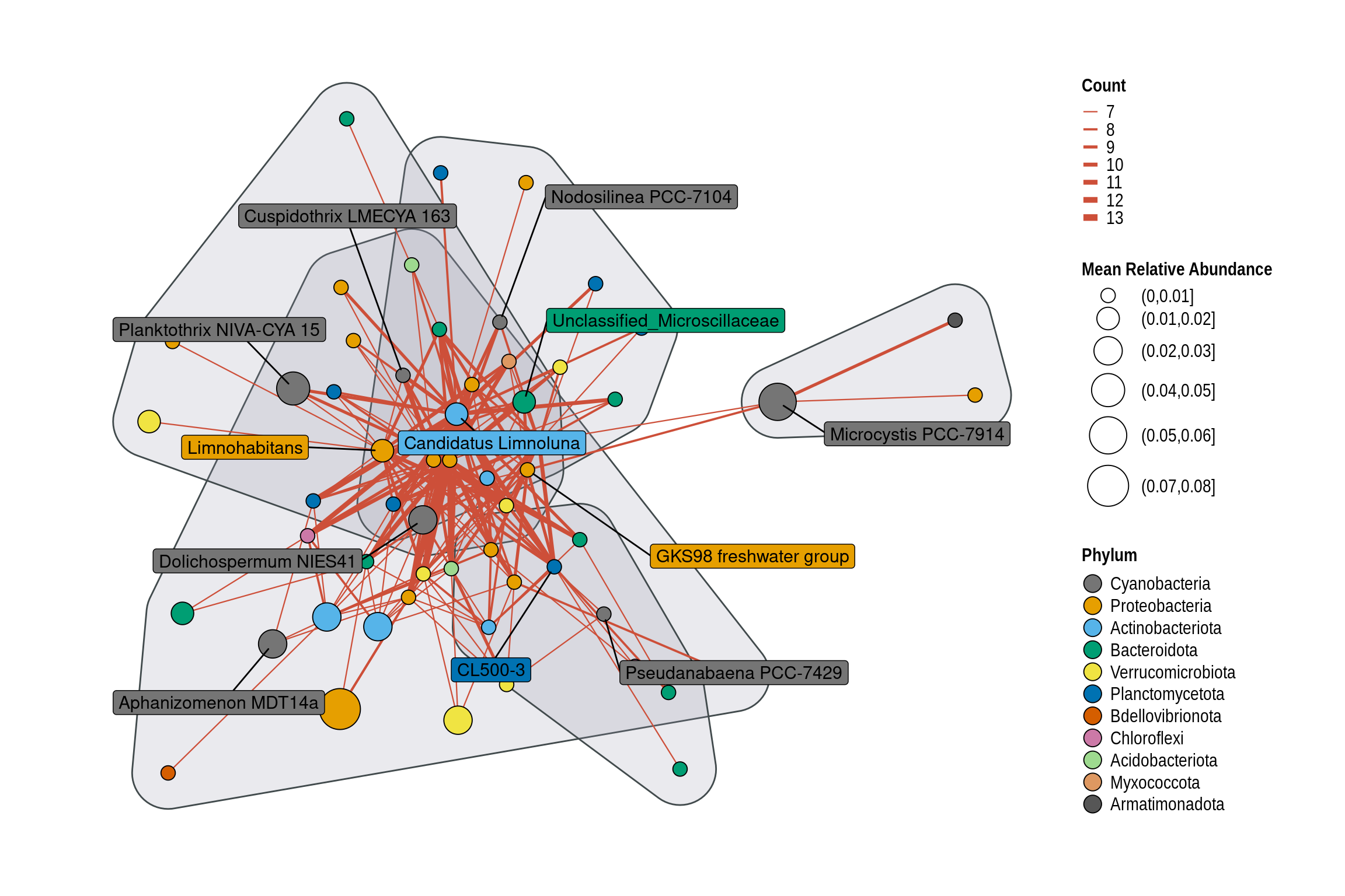

Schuyler Smith
Ph.D. Student - Bioinformatics and Computational Biology
Iowa State University. Ames, IA.