Molecular Analysis

Abiotic Factors

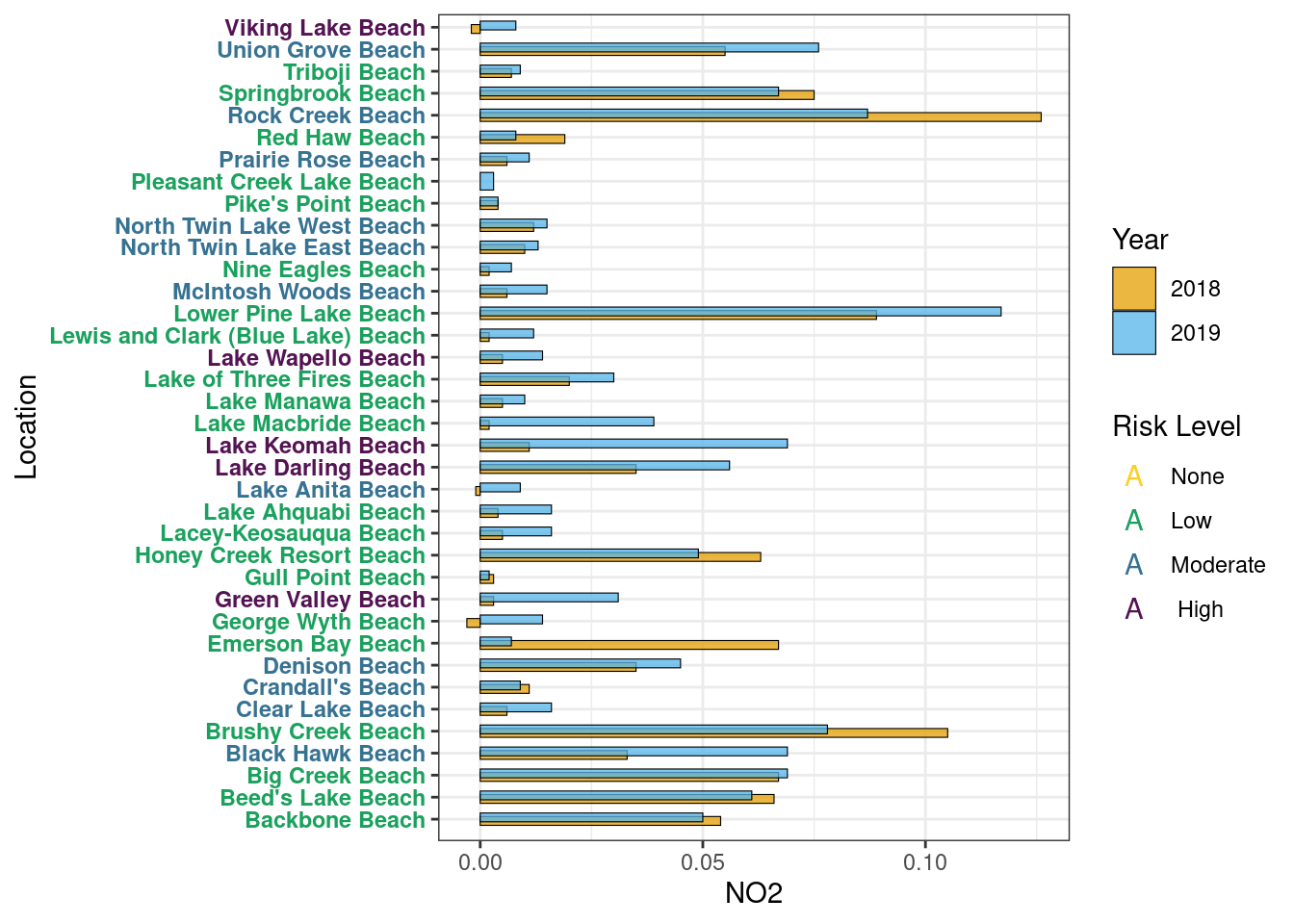
NO2

Year Average

nitrogen <- metadata[, lapply(.SD, mean, na.rm=TRUE), 
                     by=c("Location", "Year"), 
                     .SDcols=c("NO2")][order(Location)]
set(nitrogen, j = "NO2", value = round(nitrogen$NO2, 3))

Graph

Table

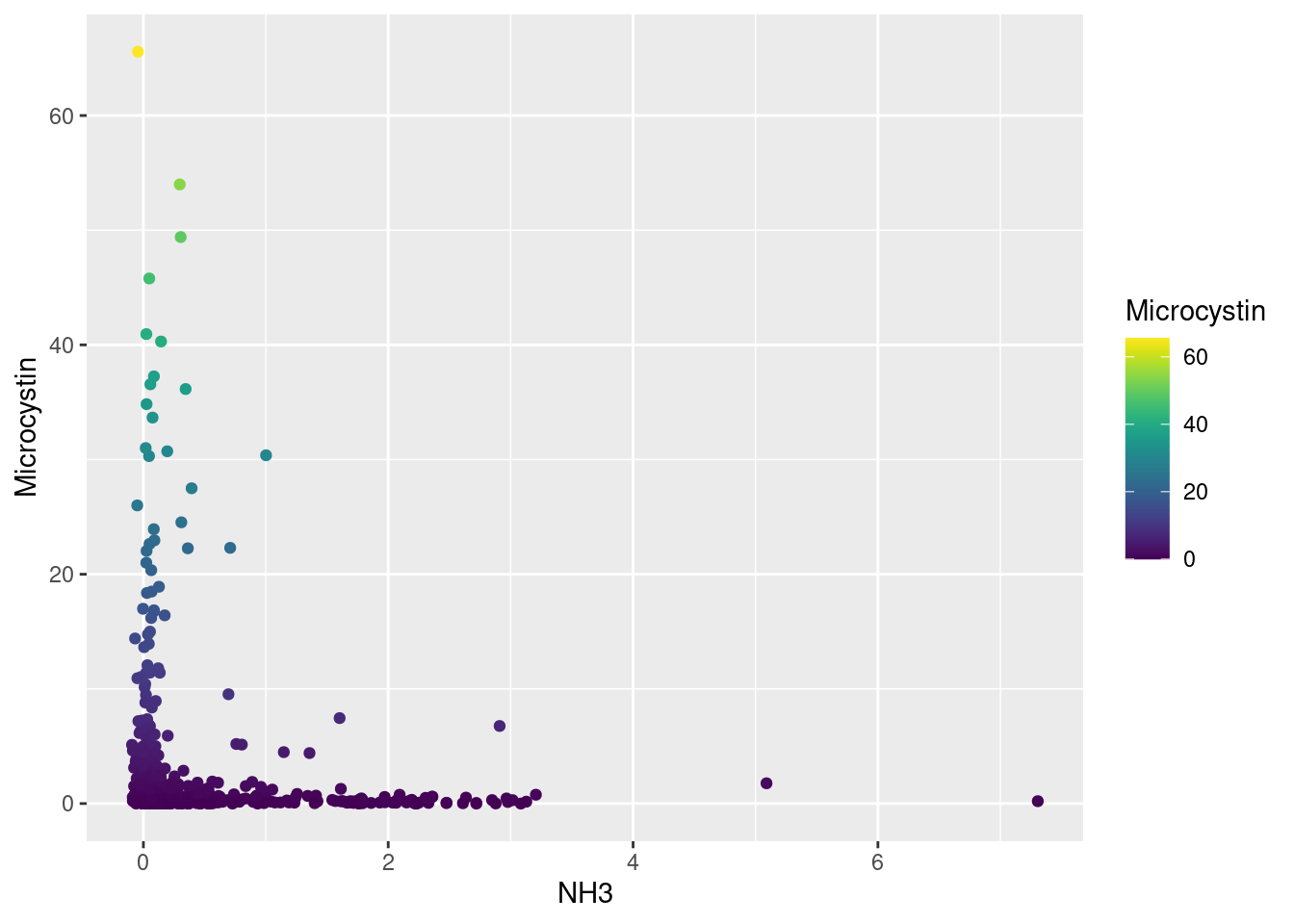
Microcystin Correlation

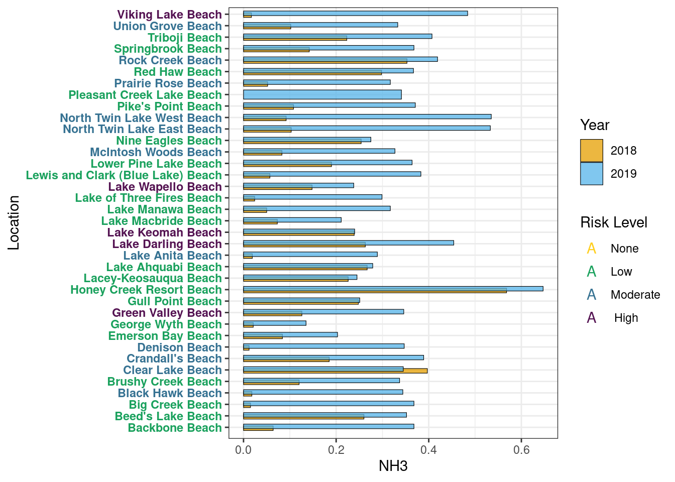
NH3

Year Average

NH3 <- metadata[, lapply(.SD, mean, na.rm=TRUE), 
                by=c("Location", "Year"), 
                .SDcols=c("NH3")][order(Location)]
set(NH3, j = "NH3", value = round(NH3$NH3, 3))

Graph

Table

Microcystin Correlation

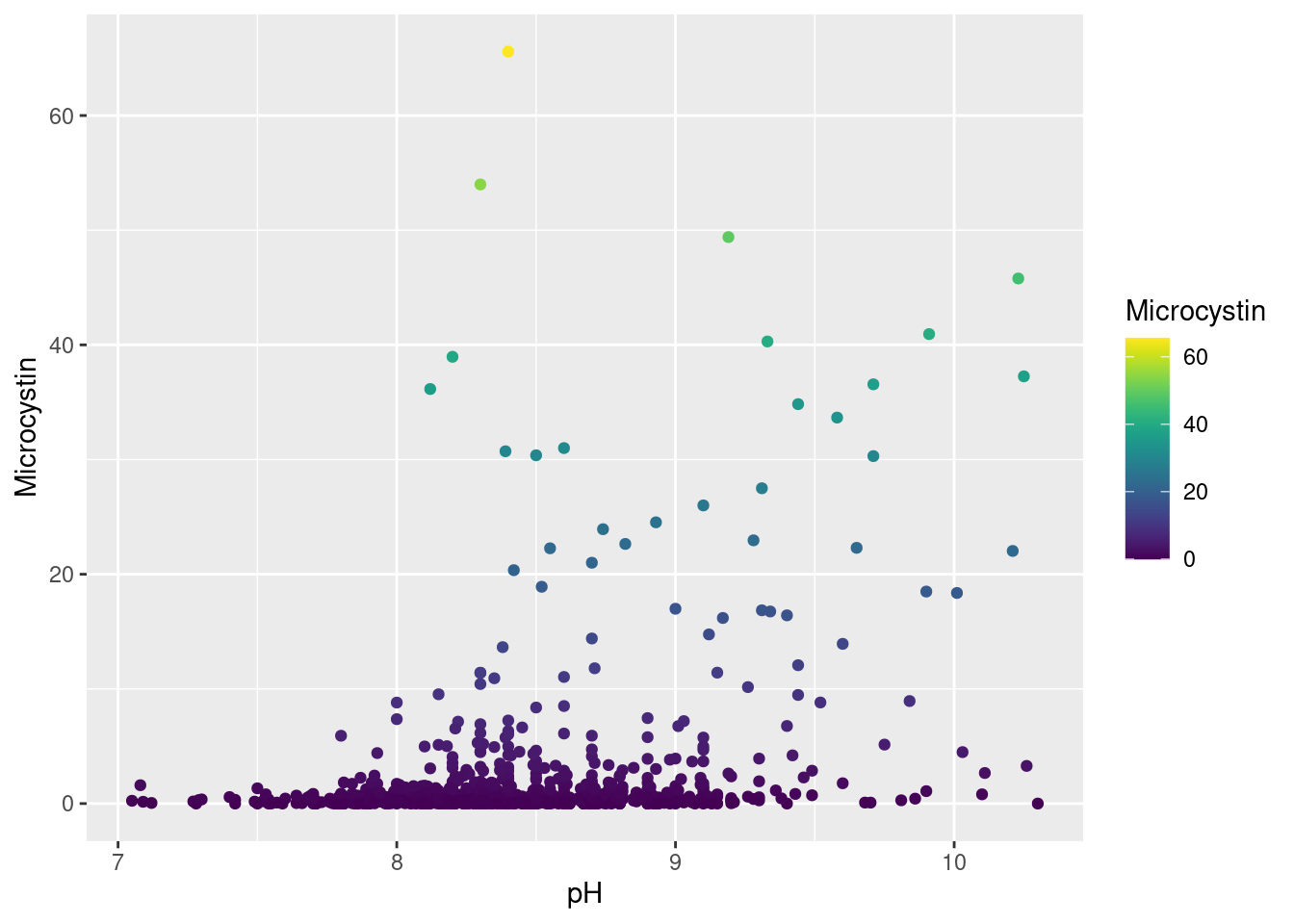
pH

Year Average

pH <- metadata[, lapply(.SD, mean, na.rm=TRUE), 
               by=c("Location", "Year"), 
               .SDcols=c("pH")][order(Location)]
set(pH, j = "pH", value = round(pH$pH, 2))

Graph

Table

Microcystin Correlation

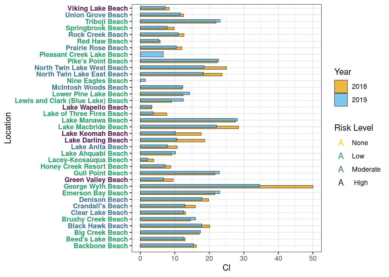
Cl

Year Average

Cl <- metadata[, lapply(.SD, mean, na.rm=TRUE), 
               by=c("Location", "Year"), 
               .SDcols=c("Cl")][order(Location)]
set(Cl, j = "Cl", value = round(Cl$Cl, 2))

Graph

Table

Microcystin Correlation

High- & Low-Risk Lakes

Weeks of Significantly Different Variables

Microcystin Levels

2018

ggplot(sam[Year == 2018], aes(x = Week, y = Microcystin)) + 
  geom_bar(stat = "identity", position = "stack", 
                        size = 0.12, width = 0.95, color = "black") + 
  facet_nested_wrap(.~ Lake_Risk + Location , scales = "free") + 
  theme_bw() +
  theme(axis.text.x = element_text(size = 8), 
        axis.text.y = element_text(size = 10), 
        axis.title.x = element_text(size = 12, face = "bold"), 
        axis.title.y = element_text(size = 12, face = "bold"), 
        axis.ticks.x = element_blank(), 
        legend.title = element_text(size = 10, face = "bold"), 
        legend.text = element_text(size = 10), 
        legend.spacing.x = unit(0.005, "npc"), 
        legend.key.size = unit(3, "mm"),
        legend.position="top",  
        panel.background = element_rect(color = "black", size = 1.5), 
        panel.spacing = unit(0.01, "npc"), 
        strip.text.x = element_text(size = 14, face = "bold"), 
        strip.background = element_rect(colour = "black", size = 1.4, fill = "white"), 
        panel.grid.major.x = element_blank()) + 
  scale_y_continuous(expand = expansion(mult = c(0.0037, 0.003), add = c(0, 0)), limits = c(0,70)) + 
  scale_x_discrete(expand = expansion(mult = 0, 
                                      add = 0.51))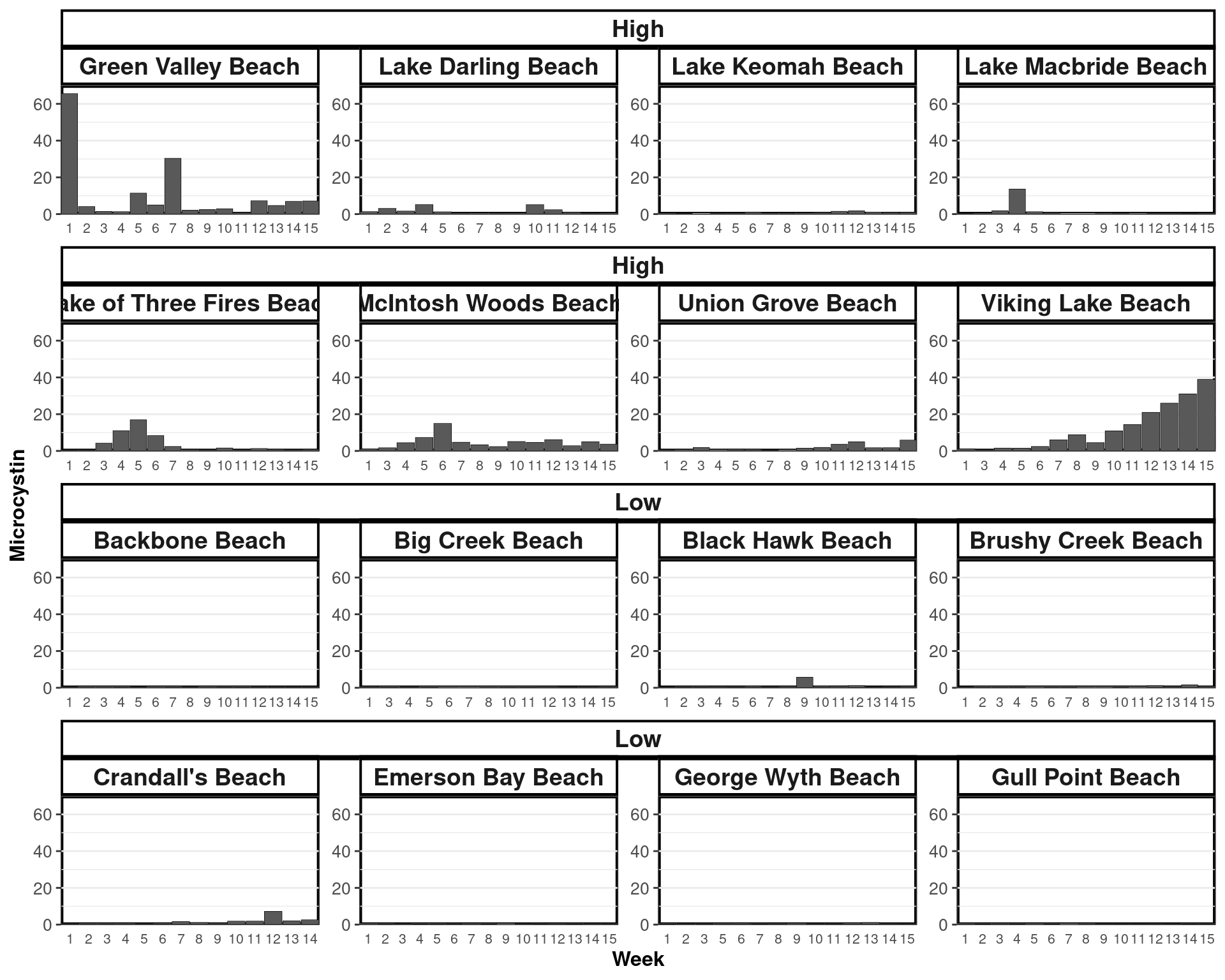

a <- data.table::copy(sam)
a[, Microcystis_x := Microcystis/max(Microcystis), by = c("Location", "Year")]
a[, Microcystin_x := Microcystin/max(Microcystin), by = c("Location", "Year")]
a <- melt.data.table(a, id.vars = c("Location", "Week", "Year", "Lake_Risk"), 
                     measure.vars = c("Microcystin_x", "Microcystis_x"))

ggplot(a[Year == 2018], aes(x = Week, y = value, 
    fill = variable))+ geom_bar(stat = "identity", position = position_dodge2(padding = 3.5), 
    size = 0.2, color = "black", alpha = 0.85, width = 0.62) + 
    facet_nested_wrap(.~ Lake_Risk + Location , scales = "free") + theme_bw() +
  scale_fill_manual(values = schuylR::create_palette(1 + length(unique(a$Year)))[-1], 
                    labels = c("Microcystin", "Microcystis")) +
  labs(y = "Relative Value", fill = "Variable") +
  theme(axis.text.x = element_text(size = 8), 
        axis.text.y = element_text(size = 10), 
        axis.title.x = element_text(size = 12, face = "bold"), 
        axis.title.y = element_text(size = 12, face = "bold"), 
        axis.ticks.x = element_blank(), 
        legend.title = element_text(size = 10, face = "bold"), 
        legend.text = element_text(size = 10), 
        legend.spacing.x = unit(0.005, "npc"), 
        legend.key.size = unit(3, "mm"),
        legend.position="top", 
        panel.background = element_rect(color = "black", size = 1.5), 
        panel.spacing = unit(0.01, "npc"), 
        strip.text.x = element_text(size = 14, face = "bold"), 
        strip.background = element_rect(colour = "black", size = 1.4, fill = "white"), 
        panel.grid.major.x = element_blank()) 

2019

ggplot(sam[Year == 2019], aes(x = Week, y = Microcystin)) + 
  geom_bar(stat = "identity", position = "stack", 
                        size = 0.12, width = 0.95, color = "black") + 
  facet_nested_wrap(.~ Lake_Risk + Location , scales = "free") + 
  theme_bw() +
  theme(axis.text.x = element_text(size = 8), 
        axis.text.y = element_text(size = 10), 
        axis.title.x = element_text(size = 12, face = "bold"), 
        axis.title.y = element_text(size = 12, face = "bold"), 
        axis.ticks.x = element_blank(), 
        legend.title = element_text(size = 10, face = "bold"), 
        legend.text = element_text(size = 10), 
        legend.spacing.x = unit(0.005, "npc"), 
        legend.key.size = unit(3, "mm"),
        legend.position="top",  
        panel.background = element_rect(color = "black", size = 1.5), 
        panel.spacing = unit(0.01, "npc"), 
        strip.text.x = element_text(size = 14, face = "bold"), 
        strip.background = element_rect(colour = "black", size = 1.4, fill = "white"), 
        panel.grid.major.x = element_blank()) + 
  scale_y_continuous(expand = expansion(mult = c(0.0037, 0.003), add = c(0, 0)), limits = c(0,70)) + 
  scale_x_discrete(expand = expansion(mult = 0, 
                                      add = 0.51))

ggplot(a[Year == 2019], aes(x = Week, y = value, 
    fill = variable))+ geom_bar(stat = "identity", position = position_dodge2(padding = 3.5), 
    size = 0.2, color = "black", alpha = 0.85, width = 0.62) + 
    facet_nested_wrap(.~ Lake_Risk + Location , scales = "free") + theme_bw() +
  scale_fill_manual(values = schuylR::create_palette(1 + length(unique(a$Year)))[-1], 
                    labels = c("Microcystin", "Microcystis")) +
  labs(y = "Relative Value", fill = "Variable") +
  theme(axis.text.x = element_text(size = 8), 
        axis.text.y = element_text(size = 10), 
        axis.title.x = element_text(size = 12, face = "bold"), 
        axis.title.y = element_text(size = 12, face = "bold"), 
        axis.ticks.x = element_blank(), 
        legend.title = element_text(size = 10, face = "bold"), 
        legend.text = element_text(size = 10), 
        legend.spacing.x = unit(0.005, "npc"), 
        legend.key.size = unit(3, "mm"),
        legend.position="top", 
        panel.background = element_rect(color = "black", size = 1.5), 
        panel.spacing = unit(0.01, "npc"), 
        strip.text.x = element_text(size = 14, face = "bold"), 
        strip.background = element_rect(colour = "black", size = 1.4, fill = "white"), 
        panel.grid.major.x = element_blank()) 

rm(a)

Schuyler Smith
Ph.D. Student - Bioinformatics and Computational Biology
Iowa State University. Ames, IA.