ARG Profile
graph_data <- primer_success
graph_data <- graph_data[Gene != 'Ref']
graph_data <- graph_data[!(Gene %in% c('16S'))]
graph_data <- merge(metadata[,c('ID', 'Sample', 'Matrix')], graph_data, by.x = 'ID', by.y = 'sample')
target_counts <- data.table(Matrix = c("Mock", "Soil-A","Soil-B","Soil-C",
                    "Swine Manure-A","Swine Manure-B", "Soil-A + Manure-A",
                    "Bovine Manure", "Effluent", "Swine Fecal", "Total"),
           Targets = c(length(unique(graph_data[Matrix == "Mock"][true_pos > 0]$Target)),
                        length(unique(graph_data[Matrix == "Soil-A"][true_pos > 0]$Target)),
                        length(unique(graph_data[Matrix == "Soil-B"][true_pos > 0]$Target)),
                        length(unique(graph_data[Matrix == "Soil-C"][true_pos > 0]$Target)),
                        length(unique(graph_data[Matrix == "Swine Manure-A"][true_pos > 0]$Target)),
                        length(unique(graph_data[Matrix == "Swine Manure-B"][true_pos > 0]$Target)),
                        length(unique(graph_data[Matrix == "Soil-A + Manure-A"][true_pos > 0]$Target)),
                        length(unique(graph_data[Matrix == "Bovine Manure"][true_pos > 0]$Target)),
                        length(unique(graph_data[Matrix == "Effluent"][true_pos > 0]$Target)),
                        length(unique(graph_data[Matrix == "Swine Fecal"][true_pos > 0]$Target)),
                        length(unique(graph_data[true_pos > 0]$Target))))
classification <- 'Class'
treatment_name <- 'Matrix'
graph_data <- melt(read_counts, id.vars = c('Class', 'Family', 'Gene', 'Target'), variable.name = 'Sample_Name')
graph_data <- graph_data[Gene != 'Ref']
graph_data <- graph_data[!(Gene %in% c('16S'))]
graph_data <- merge(metadata[,c('ID', 'Sample', 'Matrix')], graph_data, by.x = 'ID', by.y = 'Sample_Name')
graph_data <- graph_data[, sum(value), by = c('Sample', 'Matrix', 'Class', 'Family')]
set(graph_data, j = classification,
value = factor(graph_data[[classification]],
levels = c('Ref', rev(unique(graph_data[[classification]][!(graph_data[[classification]]=='Ref')])))))
setkey(graph_data, "Class", "Sample")
graph_data[, relative_abundance := round(V1/sum(V1), 4), by = c('Sample')]
set(graph_data, j = 'Matrix', value = as.character(graph_data$Matrix))
setkey(graph_data, 'Sample')
graph_data <- graph_data[!(is.na(relative_abundance))]
graph_data <- graph_data[graph_data$Matrix != 'effluent',]
graph_data <- graph_data[graph_data$Matrix != 'Effluent',]
graph_data <- graph_data[V1 != 0]
graph_data[, relative_abundance := round(V1/sum(V1), 4), by = c('Sample')]
classification_order <- setorder(graph_data[, lapply(.SD, sum, na.rm=TRUE),
by=Class, .SDcols=c("relative_abundance")], -relative_abundance)
classification_order <- classification_order[round(classification_order[[2]]*100 /
length(unique(graph_data$Sample)),1) >= 0.5,]
graph_data <- graph_data[Class %in% classification_order$Class]
set(graph_data, j = 'Class', value = factor(graph_data$Class, levels = classification_order[[1]]))
graph_colors <- schuylR::create_palette(length(levels(graph_data[[classification]])))
graph_data <- graph_data[, lapply(.SD, sum, na.rm=TRUE), by=c('Sample', "Class", 'Matrix'),
.SDcols=c("V1", "relative_abundance") ]
graph_data[, relative_abundance := round(V1/sum(V1), 4), by = c('Sample')]
set(graph_data, j = 'Sample', value = factor(graph_data[['Sample']], levels = unique(graph_data[['Sample']])))
set(graph_data, j = 'Matrix', value = factor(graph_data[['Matrix']], levels = unique(graph_data[['Matrix']])))
profile <- ggplot(graph_data,
aes_string(x="Sample", y="relative_abundance", fill=classification)) +
guides(fill=guide_legend(ncol=2)) +
scale_fill_manual(values=graph_colors, aesthetics=c("color", "fill")) +
geom_bar(stat="identity", position="stack", size=0.12, width=0.95, color="black") +
ylab("Relative Abundance") +
theme_bw() +
theme(axis.text.x = element_text(size=12, angle = 330, hjust = -0.05),
axis.text.y=element_blank(),
axis.title.x=element_blank(),
axis.title.y=element_text(size=12, face="bold"),
axis.ticks.x=element_blank(),
legend.title=element_text(size=12, face="bold"),
legend.text=element_text(size=12),
legend.spacing.x=unit(0.005, "npc"), legend.key.size=unit(6,"mm"),
panel.background=element_rect(color="black", size=1.5), panel.spacing=unit(0.01, "npc"),
strip.text.x=element_text(size=12, face="bold"),
strip.background=element_rect(colour="black", size=1.4,
fill="white"), panel.grid.major.x=element_blank()) +
scale_y_continuous(expand=expansion(mult=c(0.0037, 0.003), add=c(0, 0))) +
ggh4x::facet_nested(.~ Matrix, scales = "free", space = "free") +
scale_x_discrete(expand=expansion(mult=0, add=0.51))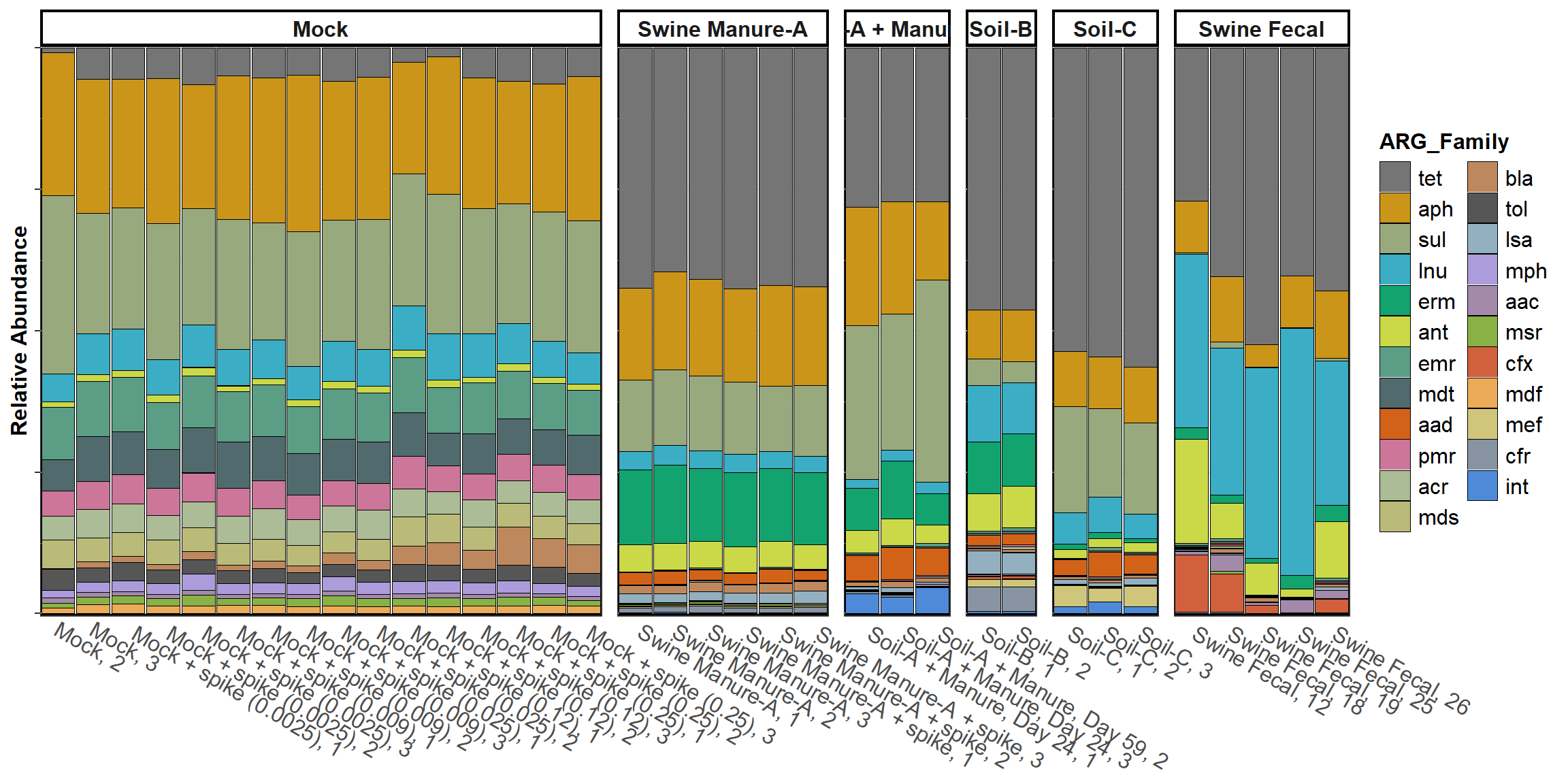
Ordination
PCA
treatment = 'Matrix'
x = 1
y = 2
method = 'bray'
circle = 0.95
graph_data <- read_counts[,-c(2,3,4)]
graph_data <- rarefy(data=graph_data[, c(1, which(colSums(graph_data[,-1])>5000)+1), with=FALSE], min(colSums(graph_data[,-1])))[,-1]
distance_matrix <- vegan::vegdist(t(graph_data), method, na.rm = TRUE)
distance_matrix[is.na(distance_matrix)] <- 0
MDS <- cmdscale(distance_matrix, k = max(c(x,y)), eig = TRUE)
graph_data <- cbind(x = MDS$points[,x], y = MDS$points[,y])
graph_data <- data.table(merge(graph_data, metadata[,c('ID', 'Sample', 'Matrix')], by.x = 0, by.y = 'ID'))

color_count <- length(unique(graph_data[[treatment]]))
graph_colors <- schuylR::create_palette(color_count)
set(graph_data, j = 'Sample', value = factor(graph_data[['Sample']], levels = unique(graph_data[['Sample']])))
set(graph_data, j = 'Matrix', value = factor(graph_data[['Matrix']], levels = unique(graph_data[['Matrix']])))

pca <- ggplot(data = graph_data, aes_string('x', 'y', group = treatment)) +
  geom_point(aes_string(fill = treatment), shape = 21,
             color = "black", size = 4, alpha = 1) + scale_fill_manual(values = graph_colors) +
  theme_bw() + theme(
    axis.line.x = element_line(colour = "black",size = 1, linetype = "solid"),
    axis.line.y = element_line(colour = "black",size = 1, linetype = "solid"),
    axis.text.x = element_text(size = 10),
    axis.text.y = element_text(size = 10),
    axis.title.x = element_text(size = 12,face = "bold"),
    axis.title.y = element_text(size = 12,face = "bold"),
    legend.title = element_text(size = 12,face = "bold"),
    legend.text = element_text(size = 12),
    legend.spacing.x = unit(0.005, "npc"),
    legend.key.size = unit(4,"mm")) +
  labs(x = paste("PCo ", x, "  (", round(sum(MDS$eig[x])/sum(MDS$eig[MDS$eig > 0]),3)*100, "%)", sep = ''),
       y = paste("PCo ", y, "  (", round(sum(MDS$eig[y])/sum(MDS$eig[MDS$eig > 0]),3)*100, "%)", sep = '')) +
  guides(fill = guide_legend(override.aes = list(size = 4))) +
  guides(fill = guide_legend(ncol = 1),
         group = guide_legend(ncol = 1))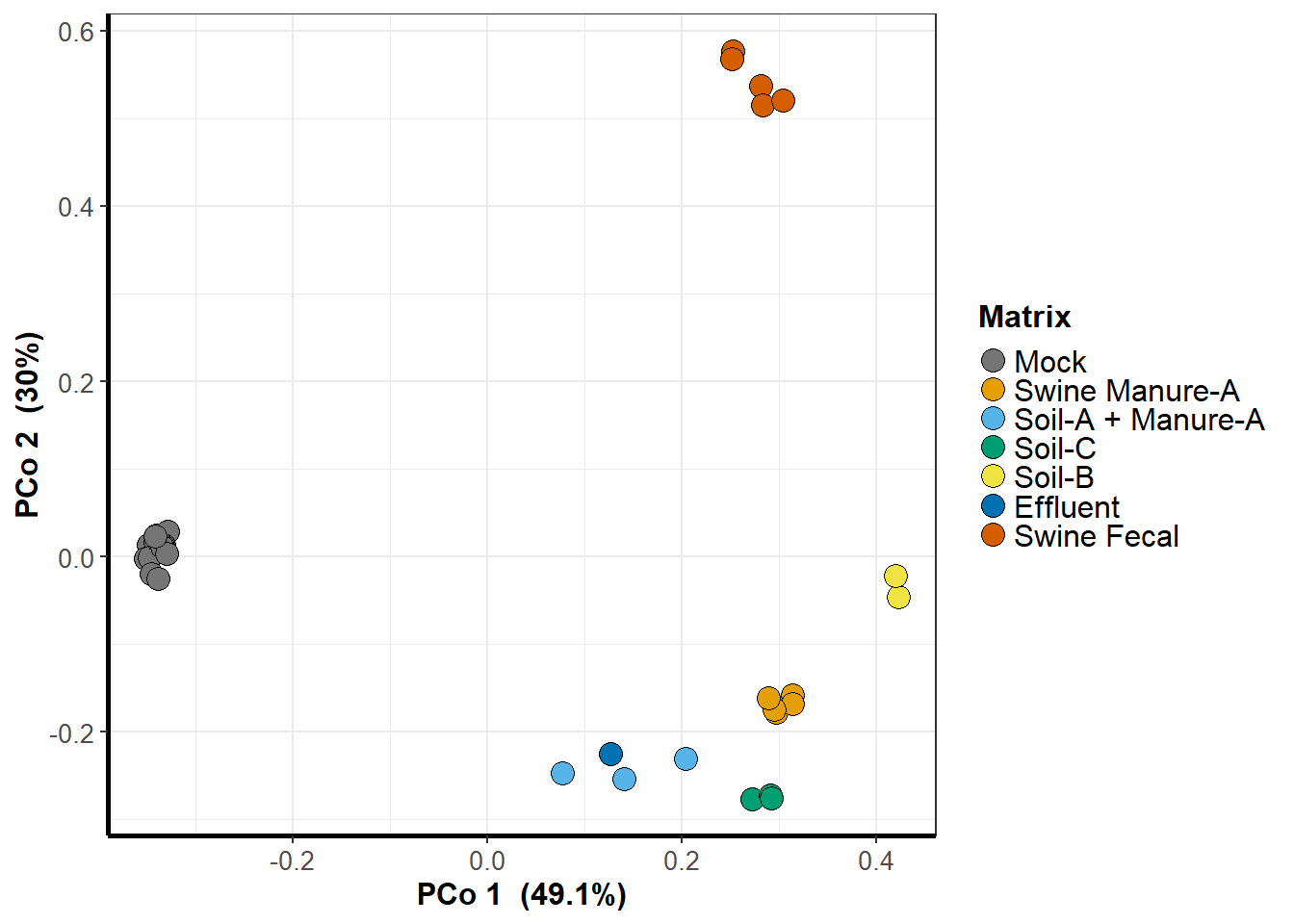
NMDS
graph_data <- read_counts[,-c(2,3,4)]
graph_data <- rarefy(data=graph_data[, c(1, which(colSums(graph_data[,-1])>5000)+1), with=FALSE], min(colSums(graph_data[,-1])))[,-1]
distance_matrix <- vegan::vegdist(t(graph_data), method, na.rm = TRUE)
distance_matrix[is.na(distance_matrix)] <- 0

MDS <- metaMDS(t(distance_matrix), autotransform = FALSE, distance = method,
  k = 3, trymax = 100, trace = FALSE)
graph_data <- data.table(merge(scores(MDS)[,c(1,2)], metadata[,c('ID', 'Sample', 'Matrix')], by.x = 0, by.y = 'ID'))

color_count <- length(unique(graph_data[[treatment]]))
graph_colors <- schuylR::create_palette(color_count)
set(graph_data, j = 'Sample', value = factor(graph_data[['Sample']], levels = unique(graph_data[['Sample']])))
set(graph_data, j = 'Matrix', value = factor(graph_data[['Matrix']], levels = unique(graph_data[['Matrix']])))

nmds <- ggplot(data = graph_data, aes_string('NMDS1', 'NMDS2', group = treatment)) +
  geom_point(aes_string(fill = treatment), shape = 21,
             color = "black", size = 4, alpha = 1) + scale_fill_manual(values = graph_colors) +
  theme_bw() + theme(
    axis.line.x = element_line(colour = "black",size = 1, linetype = "solid"),
    axis.line.y = element_line(colour = "black",size = 1, linetype = "solid"),
    axis.text.x = element_text(size = 10),
    axis.text.y = element_text(size = 10),
    axis.title.x = element_text(size = 12,face = "bold"),
    axis.title.y = element_text(size = 12,face = "bold"),
    legend.title = element_text(size = 12,face = "bold"),
    legend.text = element_text(size = 12),
    legend.spacing.x = unit(0.005, "npc"),
    legend.key.size = unit(4,"mm")) +
  labs(x = paste("NMDS-1"),
       y = paste("NMDS-2")) +
  guides(fill = guide_legend(override.aes = list(size = 4))) +
  guides(fill = guide_legend(ncol = 1),
         group = guide_legend(ncol = 1))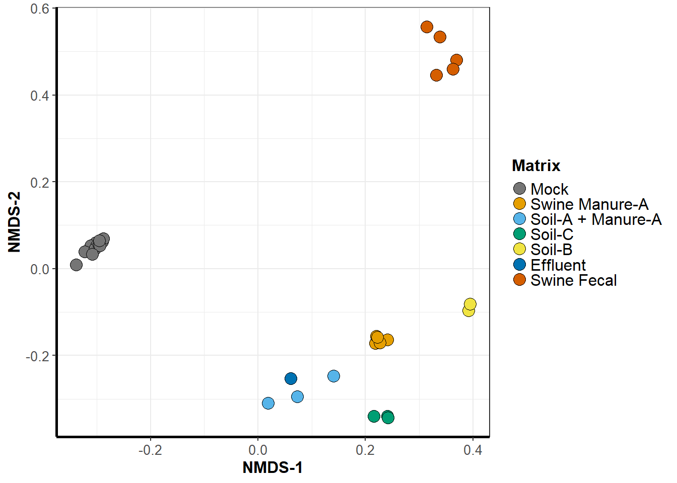
PERMANOVA
graph_data <- read_counts[,-c(2,3,4)]
graph_data <- rarefy(data=graph_data[, c(1, which(colSums(graph_data[,-1])>5000)+1), with=FALSE], min(colSums(graph_data[,-1])))[,-1]
graph_data <- graph_data[rowSums(graph_data) >=5, ]

permanova <- vegan::adonis(t(graph_data) ~ Matrix, data = metadata[`ID` %in% colnames(graph_data)])
##
## Call:
## vegan::adonis(formula = t(graph_data) ~ Matrix, data = metadata[ID %in% colnames(graph_data)])
##
## Permutation: free
## Number of permutations: 999
##
## Terms added sequentially (first to last)
##
## Df SumsOfSqs MeanSqs F.Model R2 Pr(>F)
## Matrix 6 4.8767 0.81278 10.39 0.68252 0.001 ***
## Residuals 29 2.2685 0.07822 0.31748
## Total 35 7.1452 1.00000
## ---
## Signif. codes: 0 '***' 0.001 '**' 0.01 '*' 0.05 '.' 0.1 ' ' 1
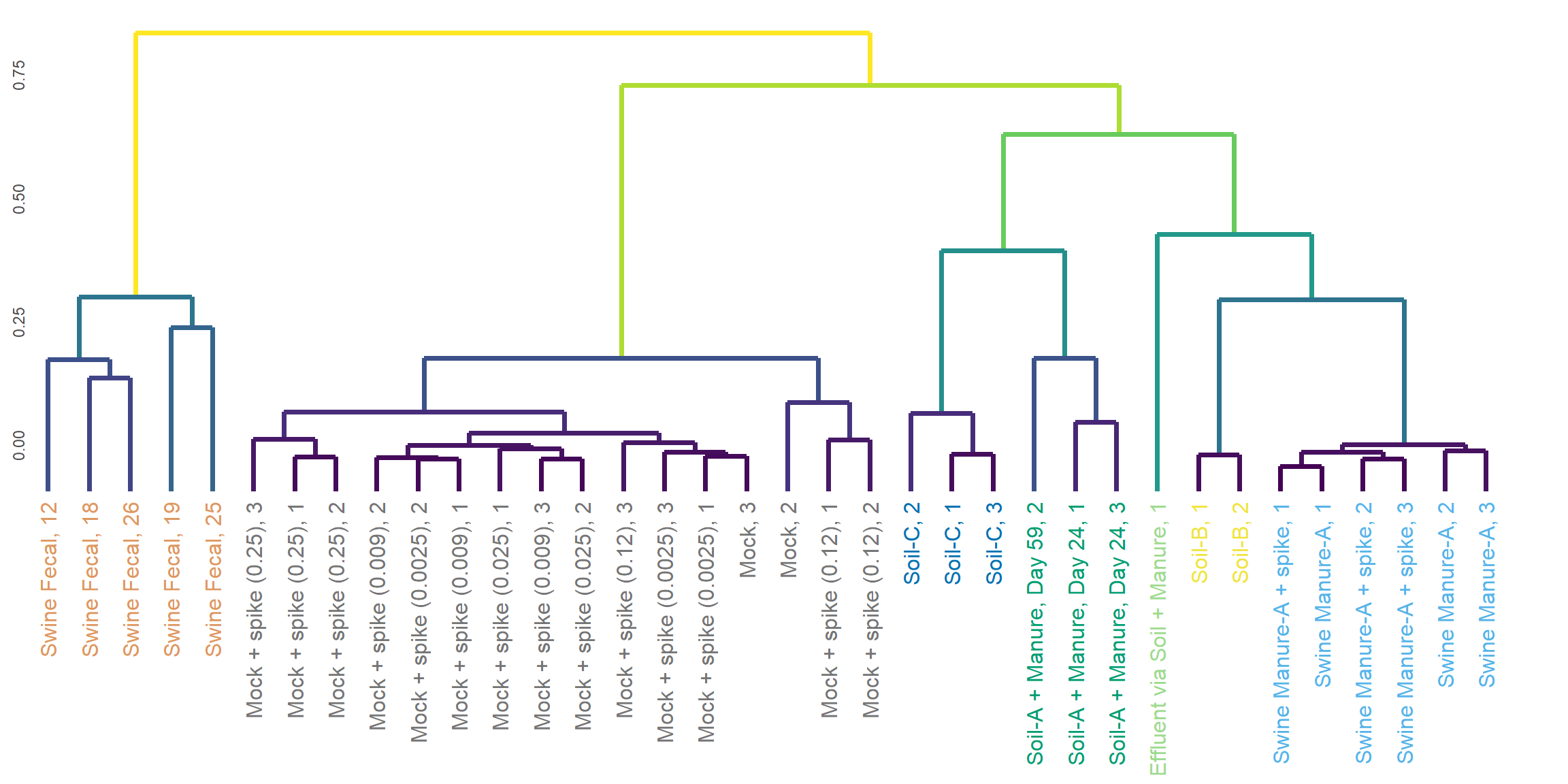
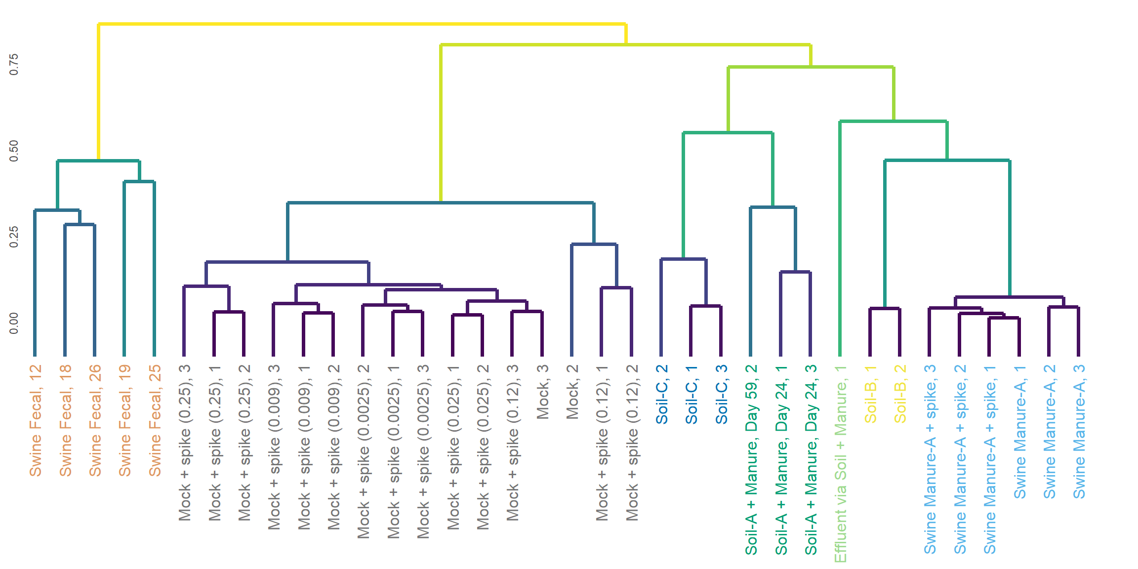
Hierarchical Clustering
for (method in c('Bray-Curts', 'Jaccard', 'Euclidean', 'Gower')){
  cat("###", method, '<br>', '\n\n')
  graph_data <- read_counts[,-c(2,3,4)]
  graph_data <- rarefy(data=graph_data[, c(1, which(colSums(graph_data[,-1])>5000)+1), with=FALSE], min(colSums(graph_data[,-1])))[,-1]
  sample_order <- colnames(graph_data)
  distance_matrix <- vegan::vegdist(t(graph_data), gsub("-.*", "",tolower(method)), na.rm = TRUE)
  distance_matrix[is.na(distance_matrix)] <- 0
  dend <- as.dendrogram(hclust(as.dist(distance_matrix), method = 'complete'))

  graph_data <- ggdendro::dendro_data(dend)
  sample_colors <- schuylR::create_palette(length(unique(metadata$Matrix))
    )[as.factor(metadata$Matrix[match(as.character(graph_data$labels$label), metadata$`ID`)])]

print(ggplot(data = ggdendro::segment(graph_data)) +
    geom_blank() +
    theme_minimal() +
    geom_segment(aes_string(x = "x", y = "y", xend = "xend", yend = "yend", color = 'y'),
                 show.legend = FALSE, size = 1.3) +
    scale_x_continuous(breaks = seq_along(graph_data$labels$label),
                       labels = as.factor(metadata$Sample[match(as.character(graph_data$labels$label), metadata$`ID`)])) +
    scale_y_continuous() +
    theme(axis.text.x = element_text(angle = 90, vjust = 0.5, hjust = 1, size = 12,
                                     margin = margin(t = -10),
                                     color = sample_colors),
          axis.text.y = element_text(angle = 90, hjust = -1,
                                     margin = margin(r = -30),),
          axis.title.x = element_blank(),
          axis.title.y = element_blank(),
          panel.grid.major = element_blank(),
          panel.grid.minor = element_blank(),
          plot.margin=unit(c(5.5, 5.5, 5.5, 5.5),"points")) + #t,r,b,l
    guides(color = guide_legend(override.aes = list(alpha=1))) +
    scale_color_gradientn(colors =  viridis::viridis(10)))
  cat('\n', '<br><br><br>', '\n\n')
}
Bray-Curts
Jaccard
Euclidean

Gower

K-Means Clustering
Optimize K
method = 'bray'
x = 1
y = 2
graph_data <- read_counts[,-c(2,3,4)]
graph_data <- rarefy(data=graph_data[, c(1, which(colSums(graph_data[,-1])>5000)+1), with=FALSE], min(colSums(graph_data[,-1])))[,-1]
distance_matrix <- vegan::vegdist(t(graph_data), method, na.rm = TRUE)
distance_matrix[is.na(distance_matrix)] <- 0

n_k = 15
graph_data <- sapply(2:n_k, function(k){
  kmeans(distance_matrix, k, nstart=20 ,iter.max = 15 )$tot.withinss
  })
graph_colors <- rep('ins', n_k-1)
graph_size <- rep(2, n_k-1)
for(i in seq(3)){
  k_value <- data.frame(k = 2:n_k, ss = graph_data, diff = c(abs(diff(graph_data)),0))
  k_value <- cbind(k_value, "percent_change" = c(0, round((k_value$diff/k_value$ss)*100)[-length(k_value$diff)]))
  if(i!=1)k_value <- k_value[(max(which(graph_colors != 'ins'))+1):nrow(k_value),]
  opt_k <- max(k_value[k_value$percent_change >= mean(k_value$percent_change) + sd(k_value$percent_change), 'k']) - 1
  graph_colors[opt_k] <- 'sig'
  graph_size[opt_k] <- 4
}
opt_k_means <- ggplot(data.frame(k = 2:n_k, graph_data), aes(k, graph_data)) +
  geom_line() +
  geom_point(size = 3, color = "black") + theme_bw() +
  scale_x_continuous(breaks = c(seq(2,14, by = 2))) +
  theme(
    legend.position = c(0.9, 0.82),
    legend.justification = c("right", "top"),
    legend.text = element_text(size = 12)
  ) +
  guides(color = guide_legend(override.aes = list(size = 4))) +
  labs(x = "Number of Clusters K", y = "Total Within-Clusters Sum of Wquares", color = "")
opt_k_means
K(3)
k = 3
treatment = 'Matrix'
MDS <- cmdscale(distance_matrix, k = max(c(x,y)), eig = TRUE)
graph_data <- cbind(x = MDS$points[,x], y = MDS$points[,y])
graph_data <- merge(graph_data, metadata, by.x = 0, by.y = 'ID')
km <- kmeans(distance_matrix, centers = k, iter.max = 10, nstart = 20)$cluster
graph_data <- cbind(graph_data, cluster =  factor(km[match(names(km), graph_data$Row.names)]))
graph_colors <- schuylR::create_palette(length(unique(graph_data[[treatment]])))
cluster_colors <- schuylR::create_palette(k, colors = 'Dark2')
k3 <- ggplot(data = graph_data, aes_string('x', 'y', group = 'cluster'))
k3 <- k3 +
  geom_point(aes_string(color = 'Matrix', fill = 'Matrix'),
              size = 5, alpha = 1) +
              scale_color_manual(values = graph_colors) +
              scale_fill_manual(values = graph_colors) +
  theme_classic() + theme(axis.line.x = element_line(colour = "black", size = 1, linetype = "solid"), axis.line.y = element_line(colour = "black",
                    size = 1, linetype = "solid"), axis.text.x = element_text(size = 10),
                    axis.text.y = element_text(size = 10), axis.title.x = element_text(size = 12,
                    face = "bold"), axis.title.y = element_text(size = 12,
                    face = "bold"), legend.title = element_text(size = 10,
                    face = "bold"), legend.text = element_text(size = 12),
                    legend.spacing.x = unit(0.005, "npc"), legend.key.size = unit(4,
                    "mm"), legend.background = element_rect(fill = (alpha = 0))) +
  labs(x = paste("PCo ", x, "  (", round(sum(MDS$eig[x])/sum(MDS$eig[MDS$eig > 0]),3)*100, "%)", sep = ''),
       y = paste("PCo ", y, "  (", round(sum(MDS$eig[y])/sum(MDS$eig[MDS$eig > 0]),3)*100, "%)", sep = '')) +
  guides(fill = guide_legend(override.aes = list(size = 4))) +
  geom_polygon(data = phylosmith:::CI_ellipse(ggplot_build(k3)$data[[1]], 'group'),
               aes(x = x, y = y, group = group), color = "black",
               alpha = 0.3, size = 0.6, linetype = 1,
fill = cluster_colors[phylosmith:::CI_ellipse(ggplot_build(k3)$data[[1]], 'group', level = 0.01)$group])_graph-1.png)
K(6)
k = 6
cluster_colors <- schuylR::create_palette(k, colors = 'Dark2')
km <- kmeans(distance_matrix, centers = k, iter.max = 10, nstart = 20)$cluster
graph_data$cluster <- factor(km[match(names(km), graph_data$Row.names)])
k6 <- ggplot(data = graph_data, aes_string('x', 'y', group = 'cluster'))
k6 <- k6 +
  geom_point(aes_string(color = 'Matrix', fill = 'Matrix'),
              size = 5, alpha = 1) +
              scale_color_manual(values = graph_colors) +
              scale_fill_manual(values = graph_colors) +
  theme_classic() + theme(axis.line.x = element_line(colour = "black", size = 1, linetype = "solid"), axis.line.y = element_line(colour = "black",
                    size = 1, linetype = "solid"), axis.text.x = element_text(size = 10),
                    axis.text.y = element_text(size = 10), axis.title.x = element_text(size = 12,
                    face = "bold"), axis.title.y = element_text(size = 12,
                    face = "bold"), legend.title = element_text(size = 10,
                    face = "bold"), legend.text = element_text(size = 12),
                    legend.spacing.x = unit(0.005, "npc"), legend.key.size = unit(4,
                    "mm"), legend.background = element_rect(fill = (alpha = 0))) +
  labs(x = paste("PCo ", x, "  (", round(sum(MDS$eig[x])/sum(MDS$eig[MDS$eig > 0]),3)*100, "%)", sep = ''),
       y = paste("PCo ", y, "  (", round(sum(MDS$eig[y])/sum(MDS$eig[MDS$eig > 0]),3)*100, "%)", sep = '')) +
  guides(fill = guide_legend(override.aes = list(size = 4))) +
  geom_polygon(data = phylosmith:::CI_ellipse(ggplot_build(k6)$data[[1]], 'group'),
               aes(x = x, y = y, group = group), color = "black",
               alpha = 0.3, size = 0.6, linetype = 1,
fill = cluster_colors[phylosmith:::CI_ellipse(ggplot_build(k6)$data[[1]], 'group')$group])_graph-1.png)
Schuyler Smith
Ph.D. Student - Bioinformatics and Computational Biology
Iowa State University. Ames, IA.